S3 Table Buckets vs Redshift

AWS released S3 Table Buckets at re:Invent 2024. They seemed a very promising technology for building data lakes: not only did they offer the ability to update and delete rows, they also provided automatic optimization and compaction. Thus avoiding the performance penalty of small tables.

At release they weren’t very usable. Athena would let you query tables, but it wouldn’t let you create them. And while you could stream data into an S3 Table using Amazon Data Firehose, you couldn’t specify the table’s schema when you created it, making that capability moot. Instead, the documentation (and intro videos) directed you to use Elastic Map Reduce (EMR). At the time, I dismissed them as “not ready for prime time”, and focused instead on the similar performance enhancements for Iceberg tables in Glue.

However, over the past year, the S3 Tables team has been making improvements, and while there are still significant limitations — for example, you can’t use CloudFormation to configure Lake Formation permissions on an S3 Table — they are much more usable. In fact, S3 Tables with Athena gives a user experience similar to traditional data warehouses such as Redshift.

This post explores that idea. Redshift is a remarkably capable tool, and it’s relatively inexpensive (at least comapared to the $3 million data warehouse that I used in the mid-90s). But it’s easy for a Redshift cluster to become a significant operational expense as it grows: one of our clients started with a small, $750/month cluster, and a year later it was over $10,000/month.

Athena, which bills based on the amount of data scanned, can offer signficant savings with well-structued data. But historically, it’s required far more work to set up a table in Athena: you have to tell it where to store the data and the format to use. And if you have a streaming data source, you can easily end up with a table that has lots of small files, resulting in poor performance.

So let’s dive in. There are a couple of examples that go along with this post; I’ll link to them in the relevant sections.

What are S3 Tables, and how are they different from any other tables stored on S3?

Behind the scenes, an S3 Table is an Iceberg table stored in a special bucket type. “Behind the scenes” is an apt description, as the “bucket” itself does not contain any data. Instead, each table has its own S3 bucket, with a long random name like 26432c23-bbae-4564-jez8hhd9x77hs96ncsw3d55zwpsd1use1b--table-s3. These buckets are also “behind the scenes” in that you can’t list the files they contain.

But that’s OK, because the Iceberg format uses a metadata file to keep track of its own list of data files, so an Iceberg-aware tool can read and write the table data. This post features Amazon Athena, but there are other tools, including Spark and Amazon Data Firehose.

Integration with the Glue Data Catalog

The Glue Data Catalog is the central repository for metadata — column definitions, table locations, and the like — in an AWS data lake. This applies to both “traditional” tables stored in S3 and those stored in an S3 Table Bucket. Athena is tighly integrated with the catalog: it uses catalog metadata to perform queries, and can add items to the catalog using CREATE TABLE (you can also manually create tables using the API, or use a crawler to create tables from uncatalogued S3 data).

There is one important difference between how the Glue Data Catalog manages S3 Tables and how it manages tables stored in a standard S3 bucket: S3 Tables are not added to the “default” catalog. Instead, once you enable integration between your S3 Table Buckets and Glue, each exist as separate catalogs. This has several remifications.

First, if you go to the Glue table listing in the Console, you won’t see your S3 Tables; it just shows tables in the default catalog. You’ll see a similar behavior using the command-line interface: aws glue get-tables has an optional --catalog-id parameter; without it you just see tables in the default catalog. To see the tables in your S3 Table Buckets, you must give a catalog ID of the form s3tablescatalog/BUCKET_NAME:

aws glue get-tables --catalog-id s3tablescatalog/example --database-name my_namespace

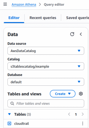
This carries through to the Athena Query Editor: within the “AwsDataCatalog” data source, you’ll find your table buckets listed (confusingly) as “catalogs” using the same naming convention.

Permissions

Actually, you won’t see anything in Athena until youd integrate S3 Tables with Lake Formation and the Glue Data Catalog. This is an easy two-click Wizard, accessed from the S3 Table Buckets page in the AWS Console. The alternative is a series of CLI commands described here.

Once you integrate Table Buckets and Lake Formation, you’ll be able to see the table bucket that you just created in the Athena Query Editor, but nobody else will. The Table Bucket owner has full permissions on the tables in the bucket, but you must grant Lake Formation permissions to anyone else.

For Athena users, this is managed in the Lake Formation Console (or via the CLI, but not, as of this writing, CloudFormation, due to a validation error). For read-only access, it’s sufficient to grant Describe permission on the catalog hierarchy and database (namespace), along with Describe and Select on the table(s). For a full read-write experience, it’s easiest to grant Super permissions at both the Database and Table level (most things that need read-write permissions will also need to create tables and perform other database maintenance tasks).

Updating Lake Formation permissions from the Console can be quite unwieldy: even with only a few users you’ll find yourself paging through many pages of permissions. You can filter by principal, but as soon as you click the “Grant” button your filter disappears and you’re back to the long list. Tag-based access control is the recommended solution, although this brings its own complexity.

Using S3 Tables with Athena

When you open the Athena query editor, you’ll see the catalog chooser on the left side of the screen. The top part lets you choose your database, and the bottom part shows you the tables in that database. When using “traditional” Glue tables, the “Catalog” field is “None”. Once you create an S3 Table Bucket, you can select that catalog from the drop-down:

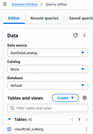
Athena catalog chooser, default Glue catalog selected Athena catalog chooser, S3 Table Bucket catalog selected

If you don’t see your Table Bucket in the Catalog selector, that means that your user does not have Lake Formation permissions to access the bucket; go back to the previous section.

Creating and Inserting

When creating “traditional” tables, stored in a standard S3 bucket, Athena requires you to specify information about the table’s storage location and format:

CREATE EXTERNAL TABLE parquet_example
(
    event_name    string,
    event_count   integer
)
STORED AS PARQUET
LOCATION 's3://my-bucket/example/'
TBLPROPERTIES
(
  'parquet.compression'='SNAPPY'
)

For Iceberg tables, the statement changes slightly: you omit EXTERNAL, and use TBLPROPERTIES to tell Athena that it’s an Iceberg table:

CREATE TABLE iceberg_example
(
    event_name    string,
    event_count   int
)
LOCATION 's3://my-bucket/example/'
TBLPROPERTIES
(
    'table_type' ='ICEBERG',
    'format'='parquet',
    'write_compression'='snappy'
)

To create the table and populate it in one step, use CREATE TABLE AS, providing location and format in the WITH clause:

CREATE TABLE iceberg_example
WITH
(
    table_type = 'ICEBERG',
    location = 's3://my-bucket/example/',
    is_external = false,
    format = 'parquet',
    write_compression = 'snappy'
)
AS
SELECT  event_name, count(*) AS event_count
FROM    cloudtrail_parquet
GROUP   BY 1

The first thing you’ll notice when creating S3 Table Bucket tables is that you don’t have to provide location or format specifications:

CREATE TABLE s3tables_example
AS
SELECT  event_name, count(*) AS event_count
FROM    cloudtrail
GROUP   BY 1

This behavior is much more like a traditional database, and for the same reason: the Table Bucket manages storage, so you don’t have to.

Cross-catalog queries

In the Athena query editor, an unqualified table name, such as in the query below, always refers to a table in the currently-selected catalog and database.

SELECT  event_name, count(*)
FROM    cloudtrail_iceberg
GROUP   BY 1
ORDER   BY 2 DESC
LIMIT   10;

THe Athena SQL Reference doesn’t indicate that SELECT can use a qualified table. However, if you choose the “Preview Table” option in Athena, you’ll get two-part table names that include the currently-selected database: "default"."cloudtrail_iceberg", and this also works in a FROM clause.

And if you’re the sort of person who reads the documentation front-to-back (or Googles for “athena qualified table names”), you’ll discover that Athena provides Federated Queries, in which it retrieves data from places other than S3, using a three-part table name: data_source.database.table.

That section of the documentation might lead you to creating a “cross-account” data source that points to an S3 Table Bucket catalog within the same account. I’m not including a link to that doc because (1) I can’t find it anymore, and (2) it isn’t necessary. Because it turns out that S3 Table Buckets are themselves a valid datasource in Athena queries:

SELECT  event_name, count(*)
FROM    "s3tablescatalog/example"."default"."cloudtrail"
GROUP   BY 1
ORDER   BY 2 DESC
LIMIT   10;

If you have an S3 table catalog selected, you can refer to your “standard” Glue catalog like this:

SELECT  event_name, count(*)
FROM    "AwsDataCatalog"."default"."cloudtrail_iceberg"
GROUP   BY 1
ORDER   BY 2 DESC
LIMIT   10;

Cross-catalog `CREATE TABLE AS`

If you’re familiar with Redshift, you’ve probably used the COPY statement: it reads data from S3 (and other sources), storing it in a Redshift table. Athena doesn’t provide COPY, but it doesn’t need to: you can create an external table in the “standard” Glue catalog to access your files on S3, and use CREATE TABLE AS or INSERT to copy that data into an S3 Table:

CREATE TABLE example
AS
SELECT * from "AwsDataCatalog"."default"."cloudtrail_parquet"

This also works in reverse, with one important caveat. For example, if you’re in the standard catalog and want to write a summary table from data stored in an S3 Table Bucket:

CREATE TABLE example
WITH
(
    external_location = 's3://my-bucket/example/',
    format = 'parquet',
    write_compression = 'snappy'
)
AS
SELECT  event_name, count(*) AS event_count
FROM    "s3tablescatalog/example"."default"."cloudtrail"
GROUP   BY 1

The caveat is that you can’t write to an Iceberg table. If you do, you’ll get the following error:

Table location can not be specified for tables hosted in S3 table buckets

I think that this is a bug in Athena; table creation and population should be separate operations, with no “bleed” from one to the other. However, it seems that Athena sees that its source data comes from an S3 Table Bucket, and ignores the fact that it’s being run in the “standard” environment. Hopefully this post turns up on the desk of an AWS project manager who also thinks it’s a bug.

In the interim, you can make this work by separating table creation and population yourself. Which works fine if you’re running those queries by hand, but some orchestation tools (such as dbt) rely on CREATE TABLE AS.

Stepping out of the Console

While querying tables in Athena is all well and good, you’re (hopefully) not going to create a data pipeline that relies on a human manually running queries. Instead, you’ll use a tool; dbt is one example that I’ve used several times, but it’s not the only one. Fortunately, Athena does give you ways to integrate such tools, but they’re not necessarily straightforward.

The basic problem is that Athena is accessed via an HTTP(S) API. This differs from Redshift, which is accessed via a TCP/IP connection using the Postgres wire protocol. Any tool that can connect to a Postgres database can also connect to a Redshift warehouse. For Athena, you must have a custom adapter that invokes your SQL using the AWS API. For example, Tableau has an Athena Connector. And AWS has created JDBC and ODBC drivers, so that tools using these standards can also connect to Athena.

The bottom line: check your tool’s documentation to see it provides a custom adaptor, or if you can use the existing JDBC or ODBC adaptors.

Glue

Glue is the primary ETL tool in the AWS ecosystem, and AWS has created an open source project that lets Glue integrate with an S3 Tables catalog. You can find an example of its use in the S3 Tables docs, but that example doesn’t quite match the README for the open-source project. In this section I’ll dig into an example Glue script.

Note: these instructions only work with Glue 5.x and above.

Permissions

Glue uses an execution role to run your scripts, and that role must have both IAM permissions and be the target of a Lake Formation grant.

The AWS documentation linked above says to attached the managed policies AmazonS3FullAccess and AmazonS3TablesFullAccess to that role. While this may be fine in a sandboxed development account, I recommend more limited grants (see the CloudFormation template from the linked example for details):

Glue Data Catalog

This consists of glue:GetDatabase and glue:GetTable, which allow retrieving table metadata, along with glue:CreateTable and glue:UpdateTable, which allows writing the metadata. These permissions can be restricted to a specific S3 bucket catalog.
Lake Formation

The only permission you need is lakeformation:GetDataAccess, which allows retrieving temporary credentials that allow access to the actual data. It can’t be restricted to individual resources.
S3 Tables

To provide read-only access, you need the s3tables:GetTable and s3tables:GetTableData permissions; these can be restricted to a single table. For read-write access you’ll need additional permissions; these are used in the example’s execution role.
S3 Data Access

These are standard permissions to read and/or write the “traditional” tables stored on S3.
S3 Script Access

This is a s3:GetObject that allows Glue to read your script from its source bucket.

In addition to these IAM permissions, you must grant Lake Formation permissions. And these do need to be wide-ranging, since your Glue scripts will not only read existing tables but create new ones.

Configuration

To enable Glue to access S3 Tables with Spark SQL, you must set several configuration parameters when creating your SparkSession:

spark = SparkSession.builder.appName("SparkIcebergSQL") \
    .config("spark.jars.packages", "org.apache.iceberg:iceberg-spark-runtime-3.4_2.12:1.4.2") \
    .config("spark.sql.extensions", "org.apache.iceberg.spark.extensions.IcebergSparkSessionExtensions") \
    .config("spark.sql.catalog.example", "org.apache.iceberg.spark.SparkCatalog") \
    .config("spark.sql.catalog.example.catalog-impl", "org.apache.iceberg.aws.glue.GlueCatalog") \
    .config("spark.sql.catalog.example.glue.id", "123456789012:s3tablescatalog/example") \
    .config("spark.sql.catalog.example.warehouse", "arn:aws:s3tables:us-east-1:123456789012:bucket/example") \
    .getOrCreate()

The important thing to note here are the spark.sql.catalog parameters. You can have multiple catalogs loaded into your workspace, each with its own name. In this case I’ve chosen the name example, so all of the parameters include that in their name. I’ve modified the configuration slightly from that in the linked S3 user guide:

….warehouse: as of this writing, the user guide shows an S3 URL, while the project README is clear that this should be the table bucket’s ARN.
….glue.id: this isn’t mentioned in the project doc, but is required to access tables. In this example, “123456789012” is my (redacted) account ID, while the trailing “example” is the name of the table bucket.
The doc also shows the parameter spark.sql.defaultCatalog, which I’ve omitted. This means that, by default, my reads and writes will be to the default Glue Data Catalog. To read or write to an S3 Table, I need to explicitly prefix with the catalog name (“example”). The result is that I can do cross-catalog operations.

A simple transformation

If I have to use Spark, I try to use Spark SQL (and I don’t ask too many questions about what it’s doing behind the scenes). Here, I run an aggregation against an S3 Table, and write it to a normal S3 bucket as Parquet (creating a table in the Glue Data Catalog along the way):

selection = spark.sql("""
                      SELECT  event_name, count(*) as event_count
                      FROM    example.default.cloudtrail
                      GROUP   BY event_name
                      """)

selection.createTempView("selection")

selection = spark.sql("""
                      CREATE TABLE IF NOT EXISTS event_counts
                      STORED AS PARQUET
                      LOCATION 's3://my-bucket/event_counts/'
                      AS SELECT * from selection
                      """)

According to the Glue job log, this took 1:17 to run using 2 DPUs, which is far longer than simply running the query in Athena. However, if you can develop your entire data pipeline as a single job, you can amortize the Glue overhead.

Performance Comparison with Redshift

The title of this post is “S3 Tables versus Redshift”, and this is the point where I compare the two in terms of performance. To do that, I used two datasets: the first is a year’s worth of Chariot’s CloudTrail data, and the second is the simulated “clickstream” data that I’ve used for several previous posts. Neither of these are truly “big data”, but in my opinion they are useful for performance analysis.

While my primary goal of these experiments was to compare S3 Tables and Redshift, I also created “traditional” Iceberg and Parquet tables as a baseline (see also my posts from 2023, comparing different Athena data stores and Athena versus Redshift.

For each dataset, I report the number of files (where applicable) and size of the table(s). For data stored in regular S3 buckets, I listed all of the files and used a spreadsheet to aggregate. For data stored in S3 Tables, I used the CloudWatch storage metrics. And for Redshift, I queried SVV_TABLE_INFO.

For each query, I show execution time and data scanned. For queries run on Athena, both values are reported in the query editor after the query completes. For Redshift, timing was reported by psql and data scanned by querying SYS_QUERY_HISTORY and SYS_QUERY_DETAIL.

I ran each query only once, primarily to avoid any issues with caching. A more rigorous test would run multiple times and average the results, throwing away high and low outliers, but this seemed like an unnecessary amount of work: barring cache effects, executing the same query twice should do the same amount of work.

CloudTrail

The reason for picking CloudTrail is that, while it doesn’t have that many rows (5,452,000 in this dataset), those rows are very wide: 27 columns, most of them containing strings, some of which are stringified JSON objects that themselves contain dozens of fields (in a few cases, exceeding the 65,535-character maximum width of a Redshift varchar). The records are relatively evenly spread by date, allowing experiments with partitioning. And the stringified JSON objects allow testing the query engine’s performance in the CPU-intensive task of parsing and extracting data from those fields.

For this test I used a year’s worth of CloudTrail events, fed into the various destinations using an Amazon Data Firehose (formerly known as Kinesis Firehose), essentially replicating this post. One big difference from that post is that I increased the Firehose batch sizes to their maximum values, which resulted in larger (and fewer) files in the data lake.

In addition to these four datasets, I also created Iceberg and S3 Tables variants that were partitioned by year and month from the event timestamp. I created these with a CREATE TABLE AS statement in Athena, after populating the base tables, and Athena produced a relatively small number of large files.

Lastly, for the Redhift table I used “even” distribution, and set the event timestamp as sort key. This should improve the performance of queries that involve date ranges, much like the partitioned Iceberg and S3 Tables variants.

File Counts and Sizes

Dataset	#/Files	Data Size (MiB)
Parquet	144	2,146
Iceberg	3,654	1,535
Iceberg, Partitioned	13	2,207
S3 Table	713	4,451
S3 Table, Partitioned	16	1,475
Redshift	n/a	9,722

The total number of files for the non-partitioned Iceberg dataset surprised me. In my post about Firhose and Iceberg from last year, the Iceberg dataset was of similar size but had only 15 files. In both cases, I waited a few days to let the compactor do its thing, but this time around it didn’t appear to have any effect. I don’t know whether that’s because my initial files were over some threshold size (due to Firehose settings), or because something has changed in the compaction algorithm since then.

After a few weeks I manully triggered compaction using the Athena OPTIMIZE statement. This produced 9 files, totalling 1,464 MiB. The numbers in this section, however, are from before that time; as such, they reflect the large number of data files, and the application of delete markers to the data.

And then there’s the Redshift storage size, which I can’t explain at all. I was expecting something at least close to the other tables, possibly even better given my use of dictionary compression for some fields. Redshift shards each field across all of its storage nodes, using 1 MB blocks, which can be an issue with smaller tables (those with a few thousand rows), but that can’t account for the 4x increase shown by these numbers.

Query 1: rowcount

This is about a simple as you can get, but it highlights a few interesting features of how both Athena and Redshift work.

SELECT  count(*)
FROM    cloudtrail_events

Dataset	Execution Time	Data Scanned
Parquet	1.08 sec	–
Iceberg	7.003 sec	106.25 MB
Iceberg, Partitioned	1.457 sec	–
S3 Table	2.541 sec	–
S3 Table, Partitioned	2.204 sec	–
Redshift	12.170 sec	138 MB

The first thing that jumps out is that Athena reports no data scanned for most of these queries. This makes sense: Parquet, which is the underlying storage format for everything except Redshift, keeps track of row counts in header data. So Athena just needed to open each of the files, read the headers, and sum the counts. Technically, there was some data scanned, but probably too low for Athena to report.

But then why was there data scanned for the base Iceberg table, and why did it take so long to run the query? I think the answer to both questions can be found in the 3,654 files that comprise the Iceberg table, and more important, that half of these files are delete markers. Since I populated these tables from Firehose, and knew that the original data had dupes, I configured the Firehose to perform merges rather than simple inserts. So, for each batch of data inserted into the table, there will be one file that contains the data, and one file that’s just delete markers for that data, to remove any existing rows with the same event_id. To compute the total number of rows, Athena has to combine all of these files to determine the actual set of rows.

This was supposed to be one of the benefits of Iceberg compaction: it could combine those deletes and inserts, producing (larger) files that contain only the “current” rows for the table. But, as I saw when looking at the log, it didn’t actually happen for the Iceberg table stored on S3 until I manully triggered compaction. And based on the execution time and amount of data scanned, it did happen for the S3 Table Bucket table, which was populated at the same time.

Lastly, there’s the exceptionally long time that Redshift took to perform the query. Running the query a second time (with the result cache disabled) only took 38 milliseconds. I don’t have a definitive answer, but my understanding of Redshift Serverless is that it uses S3 as backing store, and loads data into an in-memory cache as needed. This could account for a signifiant percentage of the 12 second query time, especially if there are a large number of files (which might happen if it stores individual 1 MB disk blocks). I reran the query again after a couple of days, and again got a 12 second execution time.

Query 2: aggregation by event name

This query hs to read all values in a single column. It is the sort of query that highlights the benefit of column store (which all of these datasets use).

SELECT  event_name, count(*)
FROM    cloudtrail_events
GROUP   BY 1
ORDER   BY 2 DESC
LIMIT   10

Dataset	Execution Time	Data Scanned
Parquet	0.908 sec	3.27 MB
Iceberg	7.891 sec	109.97 MB
Iceberg, Partitioned	2.485 sec	4.48 MB
S3 Table	2.244 sec	3.60 MB
S3 Table, Partitioned	2.143 sec	3.68 MB
Redshift	7.190 sec	278 MB

Again, the base Iceberg dataset takes more time and requires scanning more data; this will be consistent through the rest of these queries, so I won’t call it out again.

Redshift actually runs this query faster than the simple count, again indicating to me that it’s pulling blocks from S3, only some of those blocks were cached for the previous query. This has implications for production use of Redshift Serverless: if all of your queries touch the same data (for example, a set of weekly reports) than it will be exceptionally fast, but if your queries touch disjoint subsets of the data, they can be extremely slow.

I was impressed by the (small) amount of data scanned for the other four datasets. As I said above, there are 5.5 million rows in this dataset, meaning that Athena scanned less than one byte per row. If you look at the results, you’ll see that three events accounted for nearly half of the rows; clearly, Parquet (and by extension, Iceberg and S3 Tables) can apply some impressive compression.

Query 3: aggregation by event name and date range

This query should highlight the date-based partitioning for the second Iceberg and S3 Tables tables, and the sort order for Redshift.

SELECT  event_name, count(*)
FROM    cloudtrail_events
WHERE   event_time BETWEEN cast('2024-08-12 00:00:00' as timestamp)
                   AND cast('2024-08-17 23:59:59' as timestamp)
GROUP   BY 1
ORDER   BY 2 DESC
LIMIT   10

Dataset	Execution Time	Data Scanned
Parquet	1.33 sec	33.45 MB
Iceberg	8.991 sec	7.87 MB
Iceberg, Partitioned	1.315 sec	3.69 MB
S3 Table	2.839 sec	13.38 MB
S3 Table, Partitioned	3.538 sec	2.63 MB
Redshift	7.540 sec	528 MB

As expected, there’s less data scanned for the partitioned tables, although surprisingly, the base Iceberg query didn’t scan that much data either. I suspect this was because the file headers also have min/max values, and since the data was written in chronographic order, only a few files should have the desired rows. Although that theory doesn’t account for applying the delete markers, which should require reading all files; maybe a topic for additional research.

However, just scanning less data didn’t translate to faster queries: the simple Parquet table was faster than both of the partitioned tables. But since Athena costs are based on data scanned, this may be an acceptable tradeoff if you’re querying large tables.

Redshift was a surprise in that it didn’t appear to benefit from the defined sort order: it looks like Redshift read the complete data for both columns (event_name and event_time), applied the predicate to the latter, then merged and aggregated.

Query 4: extract value from stringified JSON object

This query has a high CPU component, as it parses a stringified JSON field and then extracts values from that field. Performance should be dependent on how many compute units perform the query, possibly overwhelming the time to read files.

WITH raw AS
    (
    SELECT  event_id, event_time, aws_region, source_ip_address,
            json_value(user_identity, 'lax $.userName') as user_name,
            json_value(user_identity, 'lax $.invokedBy') as invoked_by
    FROM    cloudtrail_events
    WHERE   event_name = 'AssumeRole'
    )
SELECT  coalesce(user_name, invoked_by, 'unknown'), count(*)
FROM    raw
GROUP   BY 1
ORDER   BY 2 desc
LIMIT   10

Note: the Redshift variant is slightly different: the CTE calls json_parse() to transform the stringified JSON into a SUPER object, which is then accessed by field name in the final query. This should be more efficient than the multiple calls to json_value() in the Athena version.

Dataset	Execution Time	Data Scanned
Parquet	1.246 sec	111.20 MB
Iceberg	6.853 sec	136.75 MB
Iceberg, Partitioned	2.515 sec	146.01 MB
S3 Table	3.186 sec	49.19 MB
S3 Table, Partitioned	2.953 sec	50.45 MB
Redshift	4.401 sec	60 MB

There’s not much difference in times (except for Parquet, again!); the thing that jumped out for me was that S3 Tables and Redshift scanned far less data than the Parquet and Iceberg tables. I’ll put this down to better compression.

Simulated Clickstream Data

In my experience, “clickstream” data, tracking a user’s interaction with an application, comprises by far the largest source of “big data” that a company will manage. Depending on how granular your events are, and how much data is carried in each, you could easily find yourself with billions of rows and terabytes of data.

My simulated data is nowhere near that large: the largest table has around 200 million rows, and most events have a half-dozen columns. But it is a much larger dataset than CloudTrail, and allows physical optimizations such as controlling the distribution on Redshift.

There are four tables, representing different steps in an eCommerce “purchase funnel”:

Table	#/Rows	Description
`product_page`	211,000,000	The user looks at a product.
`add_to_cart`	65,500,000	The user adds a product to their cart.
`checkout_started`	42,750,000	The user begins the checkout process.
`checkout_complete`	35,250,000	The user completes the checkout process.

Users and products are identified by UUIDs; there are 1,000,000 of the former and 50,000 of the latter.

Data Size

I generated the data as GZipped JSON files, each containing 250,000 records. I then uploaded these to S3, and created an external table in Athena to read them. I created the Parquet, Iceberg, and S3 Table representations from that table using CREATE TABLE AS queries. For Redshift, I used the COPY command to load the JSON files into tables distributed on user_id (which should make joins faster).

As before, sizes for the “traditional” S3 formats are based on downloading the listing of files; CloudWatch metrics for the S3 Tables; and SVV_TABLE_INFO for Redshift. All sizes are in MiB. I omitted the file counts from these stats because all formats had similar counts.

Table	GZipped JSON	Parquet	Iceberg	S3 Tables	Redshift
`product_page`	10,372	14,941	14,941	10,279	11,078
`add_to_cart`	3,345	4,671	4,672	2,724	8,493
`checkout_started`	2,139	3,079	3,032	1,783	6,547
`checkout_complete`	1,760	2,539	2,500	1,470	5,854

These files all benefitted from compression. The JSON files had about a 4:1 compressoin ratio, helped by each record including field names and other highly compressible boilerplate.
The Parquet-based files didn’t get quite that much of a boost: for one file that I selected arbitrarily, the equivalent CSV file was approximately 50% larger (761 MB versus 488 MB).
Since the most of the fields are UUIDs, and thus relatively uncompressible using Snappy, I didn’t expect even that much.

Query 1: top products by number of views

In my experience, these types of queries are the bread and butter of a reporting database, albeit usually either aggregated or filtered by date.

SELECT  productid, count(*) as views
FROM    product_page
GROUP   BY 1
ORDER   BY 2 desc
LIMIT   10

Dataset	Execution Time	Data Scanned
GZipped JSON	4.480 sec	10.13 GB
Parquet	1.378 sec	435.66 MB
Iceberg	1.759 sec	435.63 MB
S3 Table	3.621 sec	443.88 MB
Redshift	0.751 sec	1.17 GB

This is the sort of query that benefits from a columnar data store, since it only needs to examine one column. And this is borne out by the execution time and especially the amount of data scanned by the non-JSON datasets. The S3 Table dataset, surprisingly, took twice the time of an Iceberg table stored in S3, although it scans approximately the same amount of data. This could be a case where Athena simply didn’t have the resoures needed for the query,

And, unlike the CloudTrail data, Redshift is the clear performance winner even though it scans more data than the Athena tables.

Query 2: abandoned carts

A somewhat more complex query, which requires a join. In a real-world scenario, you would have additional sub-queries, to identify users that abandon their carts at different stages of the checkout process, as well as those who add items to a cart but never check out.

WITH
most_recent_starts AS
        (
        SELECT  userid, max("timestamp") as action_time
        FROM    checkout_started
        GROUP   BY userid
        ),
most_recent_completes AS
        (
        SELECT  userid, max("timestamp") as action_time
        FROM    checkout_complete
        GROUP   BY userid
        )
SELECT  count(*)
FROM    most_recent_starts s
LEFT OUTER JOIN most_recent_completes c
ON      c.userid = s.userid
WHERE   c.action_time < s.action_time
OR      c.action_time IS NULL;

Dataset	Execution Time	Data Scanned
Gzipped JSON	3.606 sec	3.81 GB
Parquet	4.399 sec	2.62 GB
Iceberg	6.438 sec	2.62 GB
S3 Table	8.429 sec	1.51 GB
Redshift	1.272 sec	10.28 GB

I was expecting Redshift to be the best here, and was not disappointed. The two tables are distributed on the same field (USER_ID), so rows with the same value are found on the same nodes, and the join is perfectly parallelizable. The Athena queries, by comparision, have to shuffle the data to make the join work.

What I didn’t expect was the amount of data that Redshift would scan to perform the query: nearly an order of magnitude more than the others. Fortunately, you don’t pay for data scanned by Redshift (unlike Athena).

I was also surprised that the query against S3 Table data scanned approximately 60% of the data as the queries against Parquet and Iceberg. Since the underlying data storage for S3 Tables is Parquet, it should be the same. I have no explanation.

Conclusion

I continue to be amazed by the performance of “plain old Parquet”: logically, it should be a tiny bit more performant than Iceberg, simply because there’s no need to read metadata files. However, in my tests the Parquet versions were often significantly faster than even the partitioned Iceberg dataset (which, since it was created via CTAS, consisted of a relatively small number of large data files, and only one set of metadata files). I used parquet-tools to inspect the files, and they appeared to have identical column definitions, both used SNAPPY compression, and the per-column compression stats were similar.

My best guess is that the Parquet data set was faster because it had -- counter-intuitively -- more files, but not that many more. As a result, Athena was able to increase parallelism. I may have seen equivalent times if I recreated the Parquet dataset using CTAS. Regardless, if I were building a data lake based on full-table transforms, I think I’d use Parquet by default, and only switch to Iceberg (or an S3 Table) if I had streaming input.

In terms of raw performance, I think the question of S3 Tables versus Redshift is a tossup. In some cases Redshift was faster, in others Athena was faster, but for most queries they were within a few percentage points of one-another. I see no reason that wouldn’t scale up to larger datasets, although small percentage differences can turn into large absolute differences.

A bigger issue to me is orchestration of data pipelines, the problems with mixing S3 Tables and traditional S3 datastores, and the lack of support for orchestration tools. While it seems that S3 Table Buckets manage optimization better than Iceberg tables in normal S3 buckets, that may not be a big benefit if you use an extract-load-transform pipeline that completely rebuilds downstream tables.

The bottom line is that I think S3 Table Buckets still need maturation before they’re a clear win over Redshift. But I’m hopeful that I’ll change my mind in the not-to-distant future.

S3 Table Buckets vs Redshift

What are S3 Tables, and how are they different from any other tables stored on S3?

Integration with the Glue Data Catalog

Permissions

Using S3 Tables with Athena

Creating and Inserting

Cross-catalog queries

Cross-catalog CREATE TABLE AS

Stepping out of the Console

Glue

Permissions

Configuration

A simple transformation

Performance Comparison with Redshift

CloudTrail

File Counts and Sizes

Query 1: rowcount

Query 2: aggregation by event name

Query 3: aggregation by event name and date range

Query 4: extract value from stringified JSON object

Simulated Clickstream Data

Data Size

Query 1: top products by number of views

Query 2: abandoned carts

Conclusion

Cross-catalog `CREATE TABLE AS`