
It’s possible to analyze your Glue jobs using just the logs they produce. Possible. But it’s not a pleasant task: your log messages are buried in messages from the framework, and in the case of a distributed PySpark job they’re spread between multiple CloudWatch log streams. And while there are tools such as the Spark UI that you can use to gain insight into your job’s execution, the connection between your job’s code and the tasks reported by that UI are not at all clear.
In this post I look at an alternative: AWS X-Ray, which captures and aggregates “trace segments” that capture execution time for specific sections of your code. With X-Ray, you can see where your jobs are spending their time, and compare different runs. Using X-Ray with Glue does require more work than using it with, say, Lambda, but the insights are no less valuable.
This is going to be a long post, so grab a cup of coffee. If you’d like to try out the examples yourself, you’ll find them here. Beware that you will incur AWS charges from running these examples, although they are small (less than a dollar unless you make repeated runs).
What is X-Ray?
X-Ray is a tool to profile your code: it gathers detailed statistics about execution time, so that you can focus on optimizing the things that matter.
Historically, profiling was confined to a single program, running on a single machine. The profiler repeatedly (and frequently) sampled a running program, and recorded the line of code being executed at each sample. From that, it could infer where the program spent its time: if 50% of the samples were from a single function, it was responsible for 50% of the execution time of the program.
Tracing tools such as X-Ray work differently: the program takes an active role, sending “trace segments” to a central aggregator. These trace segments hold exact start and end times for a segment of code, giving you a detailed account of where your program spends its time (provided, of course, that you’re able to accurately measure that time). Because the application sends the trace data, it’s possible to profile a distributed application: each component sends its own segments, and they’re tied together with a common “trace identifier.”
To give a concrete example, consider a chat application. When the user logs in, the application must retrieve their profile information, the topics that they’re following, and any direct messages or notifications. These three operations might be performed by separate micro-services.
Now let’s add some numbers (yes, these are made up): the average time taken by a login operation is 500 milliseconds, but the p95 time is 5 seconds. Distributed tracing can give you insight into those timings. The p95 times might be associated with users that follow lots of topics; you may be able to improve their experience by redesigning the way you store this information. Or, you might find that retrieving profile information takes 350 milliseconds for every user, and discover you’re missing a necessary index on that service’s database. The latter is almost certainly a better use of your time and energy, but you wouldn’t know to do it without that trace data.
As you might guess from my example, tracing finds a lot of use with web applications. And in the AWS world, X-Ray is tightly integrated with the components that make up a web application: Application Load Balancer and API Gateway generate trace IDs, and the X-Ray SDK makes it easy for your application to generate trace segments that are associated with this ID.
What is AWS Glue, and why is it hard to trace?
One AWS service that is not (as of this writing) tightly integrated with X-Ray is AWS Glue.
AWS Glue bills itself as a data integration service: a tool for retrieving data from some source, transforming it, and writing the transformed results to some destination. It was released in 2017, as a way to run Apache Spark jobs without spinning up an Elastic Map Reduce cluster. In 2019 it gained the ability to run stand-alone Python scripts (“shell jobs”).
Data transformation tasks would seem to be a prime candidate for tracing: who doesn’t want to know the most expensive operations in their data pipeline? Glue, however, presents some rather unique challenges.
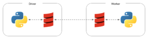
First is that, while you might write in Python, the Spark execution engine is written in Scala and runs on the Java virtual machine. When your code invokes a Spark operation, such as creating or modifying a DataFrame, that actually happens on the JVM; it’s only when the operation completes that the results (if any) are sent back to the Python environment. Using user-defined functions (UDFs) increases this complexity: each worker spins up a Python environment to run these UDFs, and PySpark ships the Python code across the network to those workers. This diagram captures the data flows:
A second complication is that Spark operations happen lazily: you can chain together a sequence of operations, and they don’t actually execute until a “terminal” operation such as count() is invoked. This means that you can’t intersperse your Spark actions with calls out to the tracer, because they will appear to take no time.
Lastly, Spark breaks apart tasks based on how the data is partitioned, and may execute pieces of different tasks concurrently.
Even with these limitations, it’s possible to use X-Ray with Spark; it just takes some thought about how the Spark job actually executes.
Permissions
As with any AWS service, X-Ray requires clients to send signed requests, and verifies that the caller has permission to execute the action. To give your Glue jobs these permissions, attach the AWS-managed policy AWSXrayWriteOnlyAccess to the job’s execution role.
Tracing a Python “shell job” with the AWS SDK
Glue “shell jobs” are Python scripts that don’t require the capabilities of Spark – or want to pay for the overhead of distributed execution. One common use case is loading and cleaning source data files.
Shell jobs have access to the boto3 library (also known as the AWS SDK), so this first example uses it to write trace information directly to X-Ray. This is the “hard way” to write traces, but it’s the only option for an “out of the box” deployment. It’s also a great introduction to exactly what goes into a trace message.
Constructing and writing trace information
As I said above, X-Ray deals with “traces” and “segments.” For this example, which converts JSON files into Avro, the trace represents the execution of the Glue job, and the segments are the sections of that job. There’s one top-level segment that tracks overall job time, and one segment for each file that is processed.
Traces and segments are identified by random (and presumably unique) IDs:
- A trace ID has the form “1-63d3ef6e-86f61d4dd1ee8baf4dc06b1e”, where “1” is a constant, “63d3ef6e” is the Unix timestamp (seconds since epoch) in hex, and “86f61d4dd1ee8baf4dc06b1e” is a 96-bit random number, also in hex.
- A segment ID is a 64-bit random number, represented as 16 hex digits (eg: “443641e51db07f73”).
The boto3 library doesn’t provide a way to generate these IDs, so I find the following function useful:
def rand_hex(num_bits):
    """ A helper function to create random IDs for X-Ray.
        """
    value = os.urandom(num_bits >> 3)
    return binascii.hexlify(value).decode()
Using this function, you can easily create trace and segment IDs:
xray_trace_id = "1-{:08x}-{}".format(int(time.time()), rand_hex(96))
xray_root_segment_id = rand_hex(64)
To report tracing information, you construct a “segment document,” which is a JSON object. It must contain the trace ID, a unique segment ID, a name for the segment, a starting time, and either an ending time or an indication that the segment is still in-progress. It may also contain a reference to a parent segment, along with various metadata fields. Here’s an example of an in-progress root segment:
xray_root_segment = {
    "trace_id" : xray_trace_id,
    "id" : xray_root_segment_id,
    "name" : job_name,
    "start_time" : time.time(),
    "in_progress": True
}
Lastly, you use the PutTraceSegments API call to write one or more segments, which are given to the API as stringified JSON:
xray_client = boto3.client('xray')
xray_client.put_trace_segments(TraceSegmentDocuments=[json.dumps(xray_root_segment)])
The sample script
For my example, I transform files from JSON into Avro, using the Python fastavro library (for more on this, see my post Avro Three Ways). These files are read from and written to S3; the bucket name and source/destination prefixes are provided as job parameters.
The core of this job is a simple loop to find all the files under the source prefix in S3 and transform each of them individually (for this example, it doesn’t matter what process() does):
s3_bucket = boto3.resource('s3').Bucket(args.data_bucket)

for src in list(s3_bucket.objects.filter(Prefix=f"{args.source_prefix}/")):
    process(s3_bucket, src.key, args.dest_prefix)
I want to record the overall script execution time, as well as the time taken to process each file. This means generating one root segment, which you saw above, as well as a sub-segment for each iteration of the loop. So the actual loop looks like this:
s3_bucket = boto3.resource('s3').Bucket(args.data_bucket)

for src in list(s3_bucket.objects.filter(Prefix=f"{args.source_prefix}/")):
    xray_start_timestamp = time.time()
    process(s3_bucket, src.key, args.dest_prefix)
    xray_child_segment = {
        "trace_id" : xray_trace_id,
        "id" : rand_hex(64),
        "parent_id": xray_root_segment_id,
        "name" : "process",
        "start_time" : xray_start_timestamp,
        "end_time": time.time()
    }
    xray_client.put_trace_segments(TraceSegmentDocuments=[json.dumps(xray_child_segment)])
Finally, we need to re-send the root segment, this time with the ending time filled in:
del xray_root_segment["in_progress"]
xray_root_segment["end_time"] = time.time()
xray_client.put_trace_segments(TraceSegmentDocuments=[json.dumps(xray_root_segment)])
The result
If you run the example script in Glue, you can go to the X-Ray page in the Console and click on the trace in the list at the bottom of the page (which should just contain a single trace). You’ll see the trace map (which isn’t very interesting) and a timeline like this:
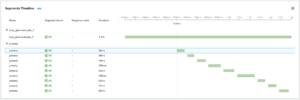
This timeline contains a lot of information. First, it shows you that the program code only took 1.6 seconds to execute – much less than the 16 seconds reported in the job’s run details (and that, combined with the 86 seconds of startup time, would be enough to convince me that Glue is the wrong choice for the job).
The trace data also shows an unexplained half-second gap between the start of the root segment and the first call to process(). This is where the script initializes boto3 clients, and retrieves the list of files to process. You could, if you want, create additional segments to capture those timings. (I haven’t done this, but would expect to to be mostly consumed by creating the first boto3 client. As I’ve written elsewhere, there’s a lot of work to create an AWS SDK client, and the script’s execution environment has only 0.0625 DPUs available)
Lastly, you can see that all of the calls to process() took about the same amount of time – the one outlier isn’t excessive. As written, the code does not differentiate between these calls, but it’s easy to add metadata to the segment, either as a nested “metadata” object, or by adding the source S3 key to the segment name.
Writing trace data with the X-Ray SDK
Creating explicit trace segments is, quite frankly, a pain. Worse, as you can see above, it hides your actual script logic. And while it’s certainly possible to write your own class that manages traces and segments, AWS already provides the X-Ray SDK.
Note: AWS is moving toward the AWS Distro for Open Telemetry (ADOT), and away from the X-Ray SDK. However, I have chosen to stick with the X-Ray SDK for this post, because I feel that ADOT is still too early in its development cycle. The documentation is filled with notes that certain APIs are not yet stable, and when I tried to walk through one of their examples – which used fixed dependency versions – I got two different import errors, depending on whether I ran in a Jupyter notebook or the Python REPL.
The biggest drawback to using the X-Ray SDK is that it’s built on the assumption that you will run an X-Ray daemon to collect traces and forward them to the X-Ray service. On paper, this makes a lot of sense: by sending traces to the daemon in UDP, you minimize the impact to the running application. And the daemon can buffer traces, making it less likely to run into (or fail because of) an X-Ray quota.
In practice, it’s not that useful: either you need to run a daemon on every server that uses X-Ray (because the default address is localhost), or you need to configure every application to use a shared server. In the case of Glue, this is a particular problem, because Glue runs in an AWS-managed VPC and doesn’t give you the opportunity to deploy a daemon locally. So if you want your Glue jobs to use the X-Ray SDK out of the box (or, for that matter, the ADOT Collector), you must run a daemon that’s exposed to the open Internet. Not something that I’m going to recommend.
A Custom Emitter
Fortunately, you don’t need to do this. The X-Ray SDK is open-source, and it’s easy to replace the internal code that reports segments to the daemon: you implement an (undocumented except for code) emitter object:
class DirectEmitter:

    def __init__(self):
        self.xray_client = None  # lazily initialize

    def send_entity(self, entity):
        if not self.xray_client:
            self.xray_client = boto3.client('xray')
        segment_doc = json.dumps(entity.to_dict())
        self.xray_client.put_trace_segments(TraceSegmentDocuments=[segment_doc])

    def set_daemon_address(self, address):
        pass

    @property
    def ip(self):
        return None

    @property
    def port(self):
        return None
The X-Ray SDK calls the send_entity() method whenever it needs to write segments. By default, this happens after every 30 completed sub-segments, but it can be configured. The passed entity is an object that accumulates segments, and as I show here, it must be converted to JSON before it’s sent to X-Ray.
Configuring the X-Ray SDK
The xray_recorder object is how your program interacts with X-Ray. When using a daemon, you can import it and use it right away. To use the custom emitter, you need to explicitly configure it:
xray_recorder.configure(
    emitter=DirectEmitter(),
    context_missing='LOG_ERROR',
    sampling=False)
You’ll notice that in addition to setting my custom emitter, I also disable sampling. When you call out to X-Ray from a web application or other high-volume service, you’ll get statistically valid results from a sample of the total calls, and avoid hitting an X-Ray quota. For Glue jobs, which aren’t run frequently, there’s no benefit to sampling. More important, if you don’t explicitly disable sampling, then the SDK makes an HTTP call to the (non-existent) daemon to retrieve sampling rules.
Also note that I set the context_missing parameter to “LOG_ERROR”. This parameter controls how the SDK behaves when it’s invoked without an open segment. The default configuration treats that as a runtime error and raises an exception. While this seems like a good idea, the SDK doesn’t play nice with threads – such as those used by the S3 Transfer Manager in boto3. By logging the error, you can either change your code to avoid threads (for example, by using get_object() rather than download_object()) or disable the warnings entirely (by configuring the recorder with “IGNORE_ERROR”).
Using the X-Ray SDK
The X-Ray SDK provides multiple ways to create (sub-) segments: you can call explicit begin/end functions, by using a decorator on a function, or as I do in this example, with a Python context manager:
with xray_recorder.in_segment(job_name):
    s3_bucket = boto3.resource('s3').Bucket(args.data_bucket)
    for src in list(s3_bucket.objects.filter(Prefix=f"{args.source_prefix}/")):
        with xray_recorder.in_subsegment("process"):
            process(s3_bucket, src.key, args.dest_prefix)
Patching dependencies
The X-Ray SDK also lets you patch some commonly-used libraries, such as boto3 or the psycopg2 database library:
patch(['boto3'])
Once patched, these libraries generate segments around their calls, so that you can see just how much time is spent in the library. While this can be very useful for a web-app – for example, to see how long your database calls take – I believe that it’s less useful for Glue jobs. If you’re dealing with large amounts of data, then it’s all too easy to generate hundreds or even thousands of segments with what seems to be an innocuous operation.
The results
The timeline for this run contains much more information, because I patched boto3. It shows the initial call to list the source files, and for each source file shows the time spent to read and write (from which the actual processing time can be inferred).
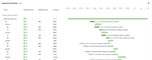
As you can also see, there’s more information attached to the S3 requests than just a segment name: you can see the operation and bucket name. This is all packed into an “aws” sub-object in the reported segment:
{
  "id": "a40cb947e9882664",
  "name": "S3",
  "start_time": 1676412336.042107,
  "end_time": 1676412336.0724213,
  "in_progress": false,
  "http": {
    "response": {
      "status": 200
    }
  },
  "aws": {
    "bucket_name": "com-chariotsolutions-kdgregory-xrayglue",
    "region": "us-east-1",
    "operation": "GetObject",
    "request_id": "BR1ABS15CHPD2WQB",
    "key": "json/addToCart/2021/08/03/c1776299-39ea-458d-82d5-f880aa1d2806.json",
    "id_2": "s7wjPADaug+DCiqS7R18yawXo5IY088Al4ZdMmYrpPO9c9TOiwjkefaVmuostxSoj7YjEvRoXV4=",
    "resource_names": [
      "com-chariotsolutions-kdgregory-xrayglue"
    ]
  },
  "namespace": "aws"
}
Tracing a PySpark driver program
Superficially, a PySpark “driver” program appears the same as the “shell job” that I used in previous examples: it’s a Python script that does stuff. The difference – and it’s a big difference – is that the “stuff” that the script does is actually performed on worker nodes in the cluster, not within the script itself.
To make this clear, consider this example:
df = spark.range(100000) \
          .withColumn('unique_id', unique_ids(df1.id)) \
          .orderBy('unique_id')
In the first line, I use the range() method to create a dataframe with a single column (id) and 100,000 rows. Spark partitions this data in preparation for distributing it to the workers in later steps (in this specific example, because it’s a single column, Spark appears to use a single partition; for other datasets, such as files read from S3, it will pick a different number of partitions).
In the second step, I add a new column to the dataset, using a Pandas UDF. I’ll dive into this function in the next section, but for now the only thing that’s relevant is that it generates a UUID for each row in the dataset. Spark calls this UDF for each partition, passing a relatively small number of rows (in my experience, around 10,000) for each invocation.
Finally, I sort the dataframe by that UUID. Not exactly something that you’d do in the real world, but it’s a good example for how Spark processes tasks.
Now the kicker: if you run that code in Glue (for example, by using the containerized environment from AWS), you’ll find that it executes almost instantaneously. It’s not until you add a “terminal” operation, such as count() or show(), that the actual chain of operations executes.
Moreover, depending on the operations, Spark might not execute all operations on all partitions. For example, show() doesn’t need all of the results, so it only requests a couple of partitions. That flows back through all of the operations: if you log every call to the UDF you will discover that it’s only called a couple of times.
Adding tracing to dataframe operations
If you want to find out how much time a particular dataframe operation takes, you must split those operations into parts, and use a terminal operation for each part. You can then wrap each part in an X-Ray segment:
with xray_recorder.in_subsegment("generate_dataframe"):
    df1 = spark.range(100000)

with xray_recorder.in_subsegment("add_unique_ids"):
    df2 = df1.withColumn('unique_id', unique_ids(df1.id))
    df2.foreach(lambda x : x) # forces evaluation of dataframe operation

with xray_recorder.in_subsegment("sort_dataframe"):
    df3 = df2.orderBy('unique_id')
    df3.foreach(lambda x : x)
Note that I used foreach() as my terminal operation. It touches every partition in the dataframe, and therefore ensures that all Spark tasks for the operation complete. It’s not very efficient to do this, but I learned the hard way that neither count() nor show() were sufficient. And you definitely don’t want to do collect()!
When you run this code, you’ll see a timeline like this:
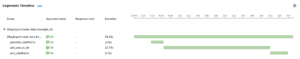
As you can see, the add_unique_ids operation took by far the largest amount of time. It’s worth diving into exactly what that operation involves, and fortunately, because it’s a Pandas UDF, we can apply X-Ray tracing to it.
Caveats
Adding tracing with this technique will reduce the efficiency of your Spark job. First, because the foreach() adds a little bit of time to the operation, as each worker scans the data it holds and then returns the results to the driver.
But more than that, breaking your Spark job into individual operations prevents the Spark scheduler from making the most effective use of resources. As an example: while I don’t know how Spark implements orderBy(), I would expect it to be a distributed merge sort: it first sorts each partition independently, and then merges them into a result (and does that only as needed by downstream operations). Because Spark performs the operation for each partition independently, some partitions might be in orderBy() while others are still in withColumn(). This improves overall throughput if withColumn() takes longer for some partitions than others.
In practice, I don’t think this is a big concern, at least for typical data transformation jobs. However, it could come into play with unbalanced groupings or joins, or with source-based partitions that are much larger than average (although that should be corrected with repartitioning).
Tracing a Pandas UDF
In the previous example, I wrote a user-defined function (UDF) to add a UUID to each row in the dataframe. In the real world you might want to do this to anonymize data, using a DynamoDB table to look up a UUID associated with a source ID rather than simply generating a new UUID for each row.
A Pandas UDF gives you the opportunity of tracing at a more granular level than the Spark operations described above. You can trace each invocation of the UDF, and see whether one invocation takes significantly more time than another. You can also capture metadata about the UDF execution, such as the number of rows that it processed.
Note: Spark provides two types of UDFs: scalar UDFs are applied to each row, and return a single result. Pandas, or vectorizable, UDFs are applied to a group of rows, and return a Pandas Series or Iterator as a result. While you could trace the execution of scalar UDFs, you will be overwhelmed by the output. Plus, they generally aren’t that complex, nor are they likely to have dramatically varying execution times.
An example UDF
Here is my Pandas UDF. It includes a short sleep in each invocation, to simulate calls out to an external service (and to make the trace graph show more than just slivers of UDF invocations).
def unique_ids(series: pd.Series) -> pd.Series:
    time.sleep(0.25)
    if series is not None:
        arr = [str(uuid.uuid4()) for value in series]
        row_count = len(arr)
        return pd.Series(arr)

unique_ids = pandas_udf(unique_ids, StringType()).asNondeterministic()
Instrumenting the job
As I mentioned at the top of this post, PySpark runs UDFs on the worker nodes. To make this happen, PySpark serializes the UDF and everything it references: global variables, functions, parameters, everything. However, there are some things that can’t be serialized, including a boto3 client object and xray_recorder.
The first of these is simple to solve: create the boto3 client inside the UDF. This is a relatively inexpensive operation, and the boto3 library maintains connections across UDF invocations. You can also create the client inside a function called from the UDF, which is what I do in this example.
The second is more of a problem, since the xray_recorder object holds the tree of trace segments; without it, you can’t attach a sub-segment into the tree. And even if you could serialize the xray_recorder and ship it to the worker, there’s no way to get the updated object back.
The best solution that I’ve found is to fall back to writing an explicit segment document using boto3. The actual UDF calls a helper function, write_subsegment(), after it completes its work:
def unique_ids(series: pd.Series) -> pd.Series:
    start_time = time.time()
    row_count = 0
    try:
        time.sleep(0.25)
        if series is not None:
            arr = [str(uuid.uuid4()) for value in series]
            row_count = len(arr)
            return pd.Series(arr)
    finally:
        write_subsegment("unique_ids", start_time, time.time(), row_count)

unique_ids = pandas_udf(unique_ids, StringType()).asNondeterministic()
The helper function creates a child segment and writes it. As you can see here, I’ve added a nested object containing additional metadata for the segment.
def write_subsegment(segment_name, start_time, end_time, row_count):
    """ A helper function so that we don't clutter the Glue code.
        """
    global xray_trace_id, xray_parent_segment_id
    xray_client = boto3.client('xray')
    xray_child_segment = {
        "trace_id" : xray_trace_id,
        "id" : generate_segment_id(),
        "parent_id": xray_parent_segment_id,
        "name" : segment_name,
        "start_time" : start_time,
        "end_time": end_time,
        "metadata": {
            "worker_ip": os.getenv("CONTAINER_HOST_PRIVATE_IP", "unknown"),
            "row_count": row_count,
        }
    }
    xray_client.put_trace_segments(TraceSegmentDocuments=[json.dumps(xray_child_segment)])
As you can see, the helper function refers to the trace and parent segment IDs using a Python global statement. The driver program assigns these variables when it creates the segment that wraps withColumn(). They are serialized and sent to the workers along with the UDF and the helper function.
with xray_recorder.in_subsegment("add_unique_ids") as segment:
    xray_trace_id = segment.trace_id
    xray_parent_segment_id = segment.id
    df2 = df1.withColumn('unique_id', unique_ids(df1.id))
    df2.foreach(lambda x : x) # forces evaluation of dataframe operation
The Result
This timeline is a little different from the previous ones: clicking on a particular segment will display details of that segment, and here I show the metadata I added earlier:
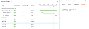
Something that jumps out from this trace is that the actual UDF invocations take a tiny slice of the time that the driver records for adding the IDs (and note that this timeline is truncated – there are far more segments than I show here). The job doesn’t even start to execute UDFs until it has been running for approximately 30 seconds. If you look at the logs for the job, you’ll see that Spark is busy spinning up workers and dispatching tasks during this time. This is why it’s important to capture driver-level trace segments in addition to UDF-level segments: you can see that optimizing that UDF is unlikely to improve the performance of your job.
Caveats
One of the drawbacks of explicitly writing segments from the UDF is that you don’t get to use all of the features of the X-Ray SDK, such as patching the boto3 library. In practice, I don’t think this is a big issue for Spark jobs: you’re typically processing a large number of rows, which means that the individual API calls would be lost in the aggregate (and, as with tracing individual scalar UDFs, would overwhelm you with detail). In my opinion, it’s better to trace larger segments, to gain an understanding of where your job spends its time. If you need more detail, either create explicit segments or use logging to capture the time taken by calls to external services.
Wrapping up
If you’ve gotten this far, you might be thinking “wow, this is one ugly hack.” And you’re not wrong. But it’s the best thing that I’ve found to-date to gain insight into the operation of a Glue job. My hope is that AWS has something in the works to provide this information with less hackage involved.
The examples that I’ve provided are intended to demonstrate the techniques, not to be the one and only way to approach the problem. For real-world use, I recommend extracting reusable code, such as the custom emitter, into its own Python module. You can then make that module available to your jobs with the --extra-py-files job parameter.
And lastly, while I’ve demonstrated how to report X-Ray segments from within your Glue jobs, that may be more than you need. CloudWatch Metrics provides a simpler, although potentially more expensive, alternative. You can report the time taken by a UDF as a metric, along with the number of rows that it processed, and view the results using a CloudWatch dashboard. And if you’re repeatedly running the same jobs, you can create an alarm based on your metrics, to let you know if a task is taking excessive time.
Can we help you?
Ready to transform your business with customized cloud solutions? Chariot Solutions is your trusted partner. Our consultants specialize in managing cloud and data complexities, tailoring solutions to your unique needs. Explore our cloud and data engineering offerings or reach out today to discuss your project.