
Over the past few weeks I’ve been experimenting with some basic machine learning. My task was to create a classifier for Slack messages. The application would be a slackbot that takes an input sentence and responds with whichever channel it believes the message should belong to. My bot only looks at three channels: #food, #fun, and #random. However, it can be easily extended to work with any number of channels.
The Network
Let’s take a look at the 3-layer neural network that I ended up with:
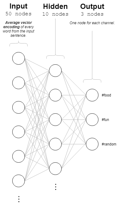
The network consists of 3 layers: the input layer, a single hidden layer, and the output layer. Let’s talk about the most important layer first: the input layer.
The Input Layer
Here you will find 50 nodes (“neurons”). This is equal to the number of dimensions in my word vector encodings. Let’s talk about what that means real quick:
Understanding Word Vectorization
As a human with (presumably) many years of experience in using words, you understand that a word is more than just a string of characters. But unfortunately for us, a string of characters is exactly how our computers see words. What if we wanted to assign meaning to words in a way that a computer can understand? Introducing: word vectors!
Imagine someone gives you a massive sheet of graphing paper and asks you to plot a point in a scatter plot for every word in the English language. They want you to make it so that more similar words are close together and more different words are far apart. So you get started, and after a little while your scatter plot starts to look something like this:
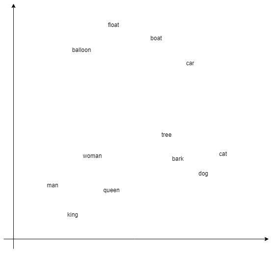
As you add more and more words you start to notice an issue: it’s getting harder and harder to demonstrate the meaningful relationships between words because you only have two dimensions to work with. That’s okay, no problem, let’s just add another dimension and start putting words onto a third axis!
So now you have a 3D point cloud of words, where every word is assigned a 3D point (or “vector”) [x, y, z]. But still…three dimensions is not really enough to portray the full depth of human language. So we can simply go and add more dimensions for our words to live in. Let’s give every word a 50-dimensional vector.
At this point, it stops being possible to visualize the scatter plot in our heads. But that’s ok, because the scatter plot isn’t for us – it’s for our computers. A computer sees a vector as just a simple list of numbers. A 3D vector is a list of 3 numbers, and a 50D vector is just a list of 50 numbers. The math is done in the same way for each!
This is the concept of word vectorization: assigning an n-dimensional vector to every word containing information about what that word means. And lucky for us, this is a problem that’s already been tackled several times! The word vectorization dataset that I’m using for my slackbot is Stanford’s GloVe: Global Vectors for Word Representation. It’s public domain and easy to use. I’m using the 50-dimensional word vector dataset that was trained on Wikipedia. It’s simply a 171 MB .txt file, where each line has a word followed by its corresponding vector (a list of 50 numbers):
austria 0.68244 0.52086 -0.24474 0.13063 -0.18005 1.1871 ...
watching -0.0049087 0.12611 0.14056 -0.16418 0.62105 ...
snow -0.044719 1.3575 0.42372 0.083063 -1.2115 0.27573 ...
pushed -0.38534 -0.8491 0.862 -0.6896 -0.20019 -0.10831 ...
elsewhere 0.80292 -0.42979 0.19956 -0.31272 -0.05101 ...
retail 0.093719 -0.50434 0.54847 0.22231 0.76707 ...
arm 0.019597 -0.99748 0.073138 -0.12371 0.76583 ...
repeatedly 0.30693 -0.87848 0.32975 -0.38582 -0.1561 ...
suffering 0.79287 0.30076 -0.18276 -0.7015 -0.39112 ...
invasion 1.0927 -1.0839 -0.10638 -0.31129 -0.41392 ...
struggle 0.145 -0.14583 0.043005 -0.35574 0.14968 ...
nfl -1.6204 0.40595 0.25878 0.37333 -0.038596 ...
This is a big oversimplification, but Stanford generated these vectors by simply scanning all of Wikipedia in 2014 and looking at how often words were found near each other. You can find details about their method, source code, and a technical paper at their website above.
Input Layer – Sentence Encoding
So now we know what word vectors are, but how do we go about using them in our input layer? Remember that our input was not individual words, but it was full sentences that we’re trying to classify with our neural network.
What we can do is take all the word vectors for every word in the sentence and simply average them. That is:
sentenceEncoding = [
    (word1.x + word2.x + ...) / num_words,
    (word1.y + word2.y + ...) / num_words,
    ...
]
So the sentence encoding is the midpoint of the vectors of all the words that make up the sentence. It’s a simple solution, but there is one drawback: you lose the context of the words’ positions. So “James likes to eat ham” has the same encoding as “ham likes to eat James”, even though those sentences mean very different things. However, this is a trade-off I was willing to make for simplicity’s sake.
So now we understand what the input layer is made of. Let’s move on to the single hidden layer.
The Hidden Layer
Hidden layers in a neural network are all the layers between the input and the output. They’re the voodoo magic used for extracting features from the input, and are the main thing that sets neural nets apart from the linear regression you used to use in math class.
For most problems, a single hidden layer is sufficient. There are several factors to consider when choosing how many neurons to include in that layer; including the size of your training dataset, the number of input neurons, and the number of output neurons. The only general rule of thumb here is that the hidden layer’s size should be between the size of the input layer and the size of the output layer. Beyond that, it’s somewhat arbitrary. I ended up going with 10 neurons in my hidden layer.
Too many neurons and your training will take longer and you could fall prey to overfitting. Too few neurons and your network might not be complex enough to properly distinguish between all the features you need it to. Experiment with different numbers and choose whichever seems to work best.
The Output Layer
This layer is the simplest layer by far. It has three nodes, one for each of the three channels (#food, #fun, and #random). The output node with the highest value after a sentence encoding is passed into the input layer is the Slack channel that our network believes the input sentence belongs in.
Training
Using a trained neural network is easy – you give it an input and you read the output. The training process is where most of the scary math you’ve probably heard about lives.
Luckily for us, every major neural network library has an implementation of backpropagation that we can use. In my case, I used Synaptic.js. The training process for Synaptic is only two lines:
net.activate(training sentence encoding);
net.propagate(LEARNING_RATE, oneHotChannel(training sentence channel));
LEARNING_RATE is just a tiny number that controls how fast the network changes as it’s being trained. I used 0.05. The function oneHotChannel just takes a channel name and converts it into the format of the output layer (“one-hot”). So:
"food" => [1, 0, 0]
"fun" => [0, 1, 0]
"random" => [0, 0, 1]
I trained the network on a sample size of 800 messages, which is admittedly very small for a machine learning problem. Nevertheless, the network performed quite well!
Results
Here are six examples to show how the resulting network classifies messages:
"Does anybody here play board games? Could I get some recommendations?"
    food: 0.04, *fun: 0.69, random: 0.34

"Can somebody recommend a recipe for cooking eggplant parmesan?"
    *food: 0.99, fun: 0.01, random: 0.07

"No, sorry, that will not work for me."
    food: 0.03, *fun: 0.69, random: 0.4

"Somebody once told me the world was gonna roll me."
    food: 0.14, *fun: 0.66, random: 0.13

"Sometimes I dream about cheese."
    *food: 0.5, fun: 0.07, random: 0.43

"The server crashed about an hour ago and we can't find the SSH keys"
    food: 0.05, fun: 0.15, *random: 0.81
Something you might notice is that the results for #fun and #random seem…well, random. The two channels are very similar to each other. This stands in contrast with #food, which has a very strong and distinct category of messages. The one difference I could see when coming up with test cases between #fun and #random was that #random seemed to show higher activation with more negativity in the input message. This could just be due to the small size of our message training set. If I were to do this again, I would choose channels that are more obviously distinct from each other.
Conclusion
Neural networks can be confusing to reason about at first, but for basic tasks like classification they really aren’t that bad! You’ll often find the hardest part of a machine learning problem will be collecting the training data. For this post, I used the Node.js Slack SDK to collect the message histories of each channel along with RXJS to gather new messages as they come in. I talked about none of that in this post, despite the fact that it’s a substantial amount of code!
The rabbit hole of machine learning runs deep, but it is navigable. You don’t need to be an expert to get great results with these tools. Sometimes a good way to learn is to simply start doing!