
Execution plans are one of the primary tools to optimize your database queries, but they can be daunting to read and understand. In this post I walk through several execution plans, explain what Redshift is doing in each, and highlight the parts of plans that indicate problems.
The dataset
To do this, I use the simulated “clickstream” data that I’ve used for my last few posts. If you want to try this out, you can find the data generator here, along with CloudFormation templates to deploy a Redshift database, and instructions for loading the data into it.
There are three tables that make up this dataset, representing three different actions that the user might take:
PRODUCT_PAGEcontains events generated by looking at a product: timestamp, user identifier, and product identifier.ADD_TO_CARTcontains events generated when the user clicks an “Add to Cart” button. It’s the same information as in the product page, along with the quantity added.CHECKOUT_COMPLETEcontains events when the user finishes the checkout pipeline. It has a timestamp and a user identifier, along with a count of the number of items in the cart and their total value.
In addition, each table has a unique identifier for the event and a column that contains the event name (this last being a “leaky abstraction” from the source data, but one that I’ve seen numerous times).
When loaded into Redshift, the data is distributed based on the userid column, because that’s used to join the tables together. It’s sorted on the timestamp column, which is a good overall practice, since most business queries are based on time.
In the real world, there would be more fields in each table, as in this Segment example, which includes extensive context for a page view. As a practical matter, I don’t think that more fields would change anything about this article: one of the Redshift’s strengths is its use of columnar data storage, which means that Redshift ill ignore any fields that aren’t used in a query.
Creating and reading an execution plan
Creating an execution plan is easy: prefix your query with “explain”:
explain
select  userid, count(*)
from    checkout_complete
group   by 1
order   by 2 desc
limit   10;
When you first look at an execution plan, it seems like a wall of text:
                                                 QUERY PLAN
-------------------------------------------------------------------------------------------------------------
 XN Limit  (cost=1000000251830.73..1000000251830.76 rows=10 width=40)
   ->  XN Merge  (cost=1000000251830.73..1000000254373.45 rows=1017085 width=40)
         Merge Key: count(*)
         ->  XN Network  (cost=1000000251830.73..1000000254373.45 rows=1017085 width=40)
               Send to leader
               ->  XN Sort  (cost=1000000251830.73..1000000254373.45 rows=1017085 width=40)
                     Sort Key: count(*)
                     ->  XN HashAggregate  (cost=147803.24..150345.95 rows=1017085 width=40)
                           ->  XN Seq Scan on checkout_complete  (cost=0.00..98535.49 rows=9853549 width=40)
(9 rows)
One of the things that gives this effect is that every step in the plan shows cost, rows, and width. Cost is, in my opinion, entirely useless; in Amazon’s own words, “Cost does not provide any precise information about actual execution times or memory consumption, nor does it provide a meaningful comparison between execution plans.”
The row count is occasionally useful. If you have a good sense of how many rows you will select (for example, you know that you have 100,000 transactions per month), then a too-large or too-small count from the plan should have you worried. Most likely, it means that you don’t have accurate statistics for the table, but might indicate that you’re missing a predicate in your WHERE clause, or have a bad join.
And lastly, width gives you a sense of how many columns you’re accessing from the table. In my example above, Redshift should only be reading the userid column, which is a stringified UUID, so a width of 40 makes sense. A larger number might indicate that you’re touching more columns than you expect, or it might, again, indicate that you need to analyze the table.
But in most cases I find it’s best to copy the plan into your text editor of choice and delete those statistics (which I’ll do for the plans in the rest of this article, as well as removing some whitespace):
XN Limit
   ->  XN Merge
       Merge Key: count(*)
       ->  XN Network
           Send to leader
           ->  XN Sort
               Sort Key: count(*)
               ->  XN HashAggregate
                   ->  XN Seq Scan on checkout_complete
My preferred way to read a plan is from the bottom up – or, more correctly, from the most indented line outwards. In this case, it’s telling me that it’s doing a sequential scan of the CHECKOUT_COMPLETE table. This is exactly what I expect: while an sequential scans are scary with an OLTP database (why isn’t it using an index?), they’re the way decision support databases work.
The next steps aggregate the data, and sort it by the count value. These steps happen on the compute nodes, but then their results are sent to the leader node for final aggregation, and application of the limit operation. As we’ll see later, this might not be an optimal step.
Joins without redistribution
Redshift performs joins in parallel, which means that the rows being joined must live on the same compute node. If you know the columns that you frequently join on, you can pick one as the distribution key: Redshift ensures that all rows with the same distribution key value live on the same node. For tables without an explicit distribution key, or which are joined using a different column, Redshift must redistribute the data to make the join possible.
In the case of my sample data, I distribute every table on the userid field. As long as I include this field in my join condition (and, for a correct query, I should!), Redshift can perform the joins in parallel. Here’s an example of a query that joins on this column:
select  atc.userid as user_id,
        max(atc."timestamp") as max_atc_timestamp,
        max(cc."timestamp") as max_cc_timestamp
from    "add_to_cart" atc
left join "checkout_complete" cc
on      cc.userid = atc.userid
group   by atc.userid
limit   10;
The execution plan for this query looks good: it performs a hash join, and DS_DIST_NONE means that it doesn’t need to redistribute any data to perform that join:
XN Limit
   ->  XN HashAggregate
       ->  XN Hash Left Join DS_DIST_NONE
           Hash Cond: (("outer".userid)::text = ("inner".userid)::text)
           ->  XN Seq Scan on add_to_cart atc
           ->  XN Hash
               ->  XN Seq Scan on checkout_complete cc
Hash joins are the most performant joins that you will see in typical decision-support queries. Redshift does have a more performant sort-merge join, but it requires that the tables use the same column for both the distribution key and the sort key. In almost all cases, it’s more valuable to use a timestamp column as a sort key, in order to limit the number of rows processed.
One quirk of how Redshift executes this query is not apparent from the plan: the last step applies the aggregation (“max”) in parallel, and then sends the results back to the leader node, which applies the limit 10. Based on my experience, it appears that the leader does not attempt to merge the results from different compute nodes: it takes the desired number of rows from a single node’s results, and then tells the other nodes to throw away their results.
Joins that redistribute
Since Redshift performs joins in parallel, if you don’t specify the join column as a distribution key then it must redistribute either the inner or the outer table in the join. This means that it it physically ships the rows across its internal network to the nodes where they can be joined. As you might guess, this can be expensive.
Redistribution often happens if you distribute your tables based on their primary keys. I’m going to step away from the clickstream data for a moment, to give the example of a (simplified) banking system:
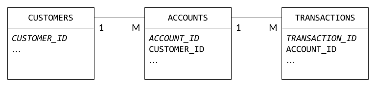
If you want to join CUSTOMERS to ACCOUNTS, then the join has to use CUSTOMER_ID; similarly, ACCOUNTS and TRANSACTIONS must be joined on ACCOUNT_ID. But if you’ve distributed based on primary key, then you’ll need to redistribute the table that holds the foreign key: ACCOUNTS when joining to CUSTOMERS, TRANSACTIONS when joining to ACCOUNTS. And note that the bigger table is always the one that gets redistributed!
Picking the correct distribution key for these three tables is a bit of an art, since there’s no column that’s present in all tables. Most likely, you’d distribute ACCOUNTS and TRANSACTIONS on ACCOUNT_ID, and pay the price when joining to CUSTOMERS. But, if you can add CUSTOMER_ID to TRANSACTIONS as part of your ETL/ELT process, then you can distribute all three tables on the same key.
Going back to my test data, what happens if the ADD_TO_CART table is distributed on eventid rather than userid? Using the same query as the previous section, the execution plan looks like this:
XN Limit
   ->  XN HashAggregate
       ->  XN Hash Left Join DS_DIST_OUTER
           Outer Dist Key: atc.userid
           Hash Cond: (("outer".userid)::text = ("inner".userid)::text)
           ->  XN Seq Scan on add_to_cart atc
           ->  XN Hash
               ->  XN Seq Scan on checkout_complete cc
In order to perform the join, Redshift redistributes all of the rows from ADD_TO_CART, signified by DS_DIST_OUTER.
So, how badly did this degrade my query? It turns out, not much: the version with the “correct” distribution key took 5.193 seconds on my 8-RPU serverless workspace, while the version with the “incorrect” distribution key took 6.301 seconds.
Partly, this is because the tables are relatively small; if they had a few hundred million rows each, you would likely see a more dramatic difference. And partly, it’s because this particular query doesn’t involve multiple columns: if your query included multiple columns from ADD_TO_CART, then you’d pay to ship all of those column values over the network.
My point here is that sometimes redistribution isn’t actually a problem. And sometimes it’s unavoidable (for example, when different queries involve different join columns). Before you change a table’s distribution key to solve a one-table redistribution, make sure that you aren’t degrading a different query. And perhaps create a copy of the table with the “correct” key to quantify the improvement before making it a permanent part of your data pipeline.
Redistribution of both tables
In my example database, all of the tables are distributed on userid. But what if they weren’t? In particular, what if they had the EVEN distribution style (which is Redshift’s default)? In that case, you’d see a query plan that looks like this:
XN Limit
   ->  XN HashAggregate
       ->  XN Hash Left Join DS_DIST_BOTH
           Outer Dist Key: atc.userid
           Inner Dist Key: cc.userid
           Hash Cond: (("outer".userid)::text = ("inner".userid)::text)
           ->  XN Seq Scan on add_to_cart atc
           ->  XN Hash
               ->  XN Seq Scan on checkout_complete cc
I have seen cases where both tables were redistributed because the query was based on an alternate – but valid – set of join columns. These tend to be extremely rare, but if you find that you’re frequently doing such joins, the best solution is to create a second copy of the tables, distributed on that alternate key.
More often, it just indicates that you haven’t assigned a key yet. This can happen as part of an extract-load-transform (ELT, as opposed to ETL) pipeline that uses the CREATE TABLE AS (CTAS) statement.
CTAS tries to be smart about picking distribution and sort keys, and uses the distribution of the tables underlying the query. However, if you’re reading from a source that doesn’t provide this information, such as a Spectrum table, CTAS defaults to EVEN distribution. Fortunately, it’s easy to specify both distribution and sort keys, as I do when setting up the example data:
create table add_to_cart
diststyle key
distkey   ( userid )
sortkey   ( "timestamp" )
as
select    *
from      ext_parquet.add_to_cart;
Redistribution that indicates an incorrect query
Query-time redistribution can also indicate a query that’s logically incorrect. Consider the following query, which is an attempt to find products that people look at but don’t add to their carts:
select  productid,
        (views - adds) as diff
from    (
        select  pp.productid  as productid,
                count(distinct pp.eventid) as views,
                count(distinct atc.eventid) as adds
        from    public.product_page pp
        join    public.add_to_cart atc
        on      atc.productid = pp.productid
        group   by pp.productid
        )
order   by 2 desc
limit   10;
At first glance, this query might seem reasonable. But logically, the join needs to include userid, because we’re comparing user actions. As written, this query vastly over-counts:: every row in PRODUCT_PAGE multiplied by every row in ADD_TO_CART with the same productid.
XN Limit
   ->  XN Merge
       Merge Key: (count(DISTINCT pp.eventid) - count(DISTINCT atc.eventid))
       ->  XN Network
           Send to leader
           ->  XN Sort
               Sort Key: (count(DISTINCT pp.eventid) - count(DISTINCT atc.eventid))
               ->  XN HashAggregate
                   ->  XN Hash Join DS_BCAST_INNER
                       Hash Cond: (("outer".productid)::text = ("inner".productid)::text)
                       ->  XN Seq Scan on product_page pp
                       ->  XN Hash
                           ->  XN Seq Scan on add_to_cart atc
DS_BCAST_INNER is the hint that something’s not right: it means that Redshift will replicate the table on all nodes. You should only see this redistribution with small “dimension” tables. In this case, it’s trying to replicate 14 million rows. This is one case where the additional plan information is useful: the “rows” statistic for this step is 109,727,636,335 (commas added for effect) – not quite a cartesian join, but close!
In this case, the the number of distinct products is relatively small (at 10,000) compared to the total number of rows. As a result, Redshift believed that broadcast would the best choice. If there were more products (say, 1,000,000), I believe that this query would use a DS_DIST_BOTH. However, it would be equally incorrect.
Overloading the leader node
The Redshift leader node does a lot of work: it handles all communications with clients, parses SQL queries and packages up work for the compute nodes, and handles any cross-cluster aggregations. This last function can overburden the leader, especially in a large cluster.
Here’s an example of a simple query that finds the top ten best-selling products for the current month:
select  productid, sum(quantity) as units_added
from    public.add_to_cart
where   "timestamp" between date_trunc('month', sysdate) and sysdate
group   by productid
order   by units_added desc
limit   10;
On my example data, this query runs very quickly, but there’s a potential problem hidden in its execution plan:
XN Limit
   ->  XN Merge
       Merge Key: sum(quantity)
       ->  XN Network
           Send to leader
           ->  XN Sort
               Sort Key: sum(quantity)
               ->  XN HashAggregate
                   ->  XN Seq Scan on add_to_cart
                       Filter: (("timestamp" >= '2023-06-01 00:00:00'::timestamp without time zone) AND ("timestamp" <= '2023-06-12 21:02:09.736206'::timestamp without time zone))
So what’s the problem? As you read this query from the bottom up, you can see the compute nodes aggregate their own data in parallel. For example, compute-0 might determine that product “123” has 12 adds, while compute-1 might say it has 182. There will be one such list for every compute node, and the list will have one row per unique product ID.
On my sample data, with 10,000 products and only a few compute nodes, this isn’t a problem. But what if you have 1,000,000 products, and a 16 node cluster? In that case, the leader node now has to aggregate 16,000,000 rows, ultimately selecting 10 of them.
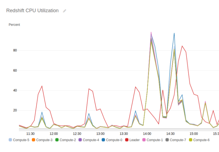
The best way to see leader overload is via CloudWatch Metrics. In the image below, individual queries are shown by jumps in CPU, and the leader node CPU consumption is shown by a red line. The first three queries aren’t great: the leader node is doing more work than the compute nodes. But the fourth query is a real problem: the red line of the leader node is offset from the rest of the nodes, meaning that the leader node isn’t able to start its work until the compute nodes have finished theirs.
If you have a large number of queries that perform such actions, then one solution is to create a separate copy of the table that’s distributed by productid. This copy would be used as a fact table for queries that do product-based aggregation, and not joined to other tables. More likely, such queries are infrequent and don’t consume a lot of resources; just let them go.
Next steps
At this point, you might be thinking “great, I can read a plan, but which plans do I read?”
This is where Redshift’s performance monitoring views come in: you start by identifying queries that take “a long time to run” using the SYS_QUERY_HISTORY view. This view contains runtimes and query text, which you can paste directly into an EXPLAIN (assuming that it isn’t truncated). As you dive deeper into query analysis, you can also use the SYS_QUERY_DETAIL view to look at how long each of the steps in your query actually took, the number of bytes it processed, and how much IO it required.
Those two tables give you a wealth of information, and if you’re running on a Provisioned cluster you have even more. Digging into those tables will be a good topic for a future post; there’s certainly a lot of data there that isn’t so easy to interpret.
Along with possibly changing your queries based on the execution plans, I highly recommend reading the list of best practices contained in the Redshift Developer Guide. Several of the practices it describes, such as using the same filter conditions (eg, timestamp) on all tables in a join, are not obvious to someone coming from an OLTP background.
Can we help you?
Ready to transform your business with customized data engineering solutions? Chariot Solutions is your trusted partner. Our consultants specialize in managing software and data complexities, tailoring solutions to your unique needs. Explore our data engineering offerings or reach out today to discuss your project.