
My last post used a Lambda with PyArrow to aggregate NDJSON files and convert them to Parquet. This is, I think, a simple and performant solution. It would be my first choice for a programmatic solution, easily beating Glue for all but the largest workloads. But what about a non-programmatic solution?
Amazon Athena has the ability to write data as well as read it, which means that we could perform the transform using SQL. Which in turn means that we could use a SQL orchestration tool such as dbt to perform this and other transformations as part of an overall data pipeline, with no need to manage a separate programmatic deployment.
While this works, and can be quite performant, there are a few stumbling blocks along the way. To highlight these, I’ll again aggregate CloudTrail log files.
First Steps: CREATE TABLE AS (CTAS)
The CREATE TABLE AS statement creates a new table from a SELECT statement. Here’s a simple example, which extracts a few of the top-level fields from the daily aggregation table created in my earlier post:
CREATE EXTERNAL TABLE cloudtrail_ctas
WITH (
        format            = 'parquet',
        external_location = 's3://com-example-data/cloudtrail_ctas/',
        write_compression = 'SNAPPY'
) AS
select  eventid             as event_id,
        requestid           as request_id,
        eventtime           as event_time,
        eventsource         as event_source,
        eventname           as event_name,
        awsregion           as aws_region,
        sourceipaddress     as source_ip_address,
        recipientaccountid  as recipient_account_id,
        useridentity        as user_identity,
        resources           as resources
from    default.cloudtrail_daily;
I ran this query against a year’s worth of data, 7,703,861 CloudTrail events. Using the daily aggregation files from my previous post, it took 17.392 seconds to run and scanned 1.99 GB. It produced 30 files, of approximately 20 MB each.
I also ran it against the raw CloudTrail logfiles for that same year. The first two attempts failed, because they exceeded S3’s request rate. S3 scales request rates when under load, so the query succeeded on the third try. It took 3 minutes and 20.832 seconds to run, scanning 3.09 GB of data.
I call this out because it’s the first stumbling block of using Athena in this way: if you have lots of small files in your repository, you’ll need to either perform an initial aggregation, rerun the query until it succeeds, or use a partitioning scheme to run the query in chunks.
And that brings up the second stumbling block: CTAS queries can only be run once. To run a second time, you must delete the table definition and the table’s data in S3. If you just delete the table, your query will fail with the error code HIVE_PATH_ALREADY_EXISTS.
INSERT-SELECT
An alternative is to create the table and then insert rows into it. The table definition has to tell Athena not only the field names and types, but where the files should be stored and what format they use. Note that the DDL below omits most of the columns for brevity, but shows the rest of the table configuration.
CREATE EXTERNAL TABLE cloudtrail_athena (
        event_id                STRING,
        request_id              STRING,
        -- a bunch of other fields
)
ROW FORMAT SERDE 'org.apache.hadoop.hive.ql.io.parquet.serde.ParquetHiveSerDe'
STORED AS PARQUET
LOCATION 's3://com-example-data/cloudtrail_athena/'
TBLPROPERTIES (
    'classification'            = 'parquet'
);
WIth the table created, we populate with another query:
insert  into cloudtrail_athena (
        event_id,
        request_id,
        -- a bunch of other fields
)
select  eventid,
        requestid,
        -- a bunch of other fields
from    default.cloudtrail_daily;
One problem with an INSERT is that it’s very much not idempotent. Each time you run the query, it will insert a new batch of rows into the destination, whether or not they’re already there.
In some cases you can make the query idempotent, by adding a test on a unique ID. For example, with CloudTrail data:
select  eventid,
        requestid,
        -- ...
from    default.cloudtrail_daily
where   eventid not in (select event_id from cloudtrail_athena);
In other cases, you may not be able to do this quite so easily. Some data streams don’t have primary key fields. In other cases, you might have so much data that the subquery is infeasible (although I think that might be more theoretical than real; I haven’t yet found such a dataset).
Data Conversion
Perhaps the biggest stumbling block in using Athena is when you have data of one type, but want to store it as a different type. For example, in the CloudTrail data the eventTime field is a string holding an ISO-8601 timestamp. Plus, there are several “complex” fields: userIdentity and tlsDetails are structs, while resources is an array of structs.
The first conversion seems very straightforward: Athena provides the from_iso8601_timestamp() function to parse ISO-8601 timestamps. However, this function returns a timestamp with timezone, while the Athena TIMESTAMP type doesn’t have a timezone (it’s presumed to be UTC). The solution is to explicitly cast the parsed timestamp into an Athena TIMESTAMP value:
cast(from_iso8601_timestamp(eventtime) as timestamp),
Athena can also handle well-defined structs and arrays (meaning that all components are known). However, when you write a nested field to Parquet, Athena creates separate columns for each component field. On the one hand, this is a good thing: it’s much more performant than extracting data from stringified JSON. On the other, it can make your files much larger, especially if some fields are only present in a small number of records.
But, for consistency with my monthly aggregation from the previous post, I convert these fields into JSON strings. This is a two-step process: casting the struct or array into JSON (which is a runtime-only type), then using json_format() to turn that object into a string:
json_format(cast (useridentity as JSON)),
Partitioning
Partitioning is the organization of your data into hierarchical “folders” based on some term that’s involved in most or all queries. For example, in the previous posts I partitioned by date: the file s3://com-example-data/2024/01/01/000000.ndjson contained records from January 1 2024. This can provide enormous speedup to any queries that look at only a range of dates, because Athena only reads the files with the appropriate prefix. The speedup depends on the query date range and how much data you have: selecting one month from four years of data should give you a nearly 98% boost.
With Athena, you specify partition columns when creating the table:
CREATE EXTERNAL TABLE cloudtrail_athena (
        -- column definitions
)
PARTITIONED BY (
        year                    string,
        month                   string
)
You must then provide the partitioning values when inserting into the table. For example, my daily aggregation table has fields for year, month, and day; when inserting into the new table, I simply omit the last of these:
insert  into cloudtrail_athena (
        year,
        month,
        event_id,
        -- remaining fields
)
select  year,
        month,
        eventid,
        -- remaining fields
from    default.cloudtrail_daily
where   eventid not in (select event_id from cloudtrail_athena)
When using INSERT INTO with partitions, Athena has a few quirks. First, it uses “Hive-style” partition naming, which includes the column name as part of the prefix. So, the files produced by this query will have names that start with s3://com-example-data/cloudtrail_athena/year=2024/month=01/.
Second, Athena writes partition information to the Glue data catalog, and then retrieves the list of partitions when it runs a query. This isn’t likely to be a problem with month/year partitioning, which may have at most a few hundred partitions. It can be a big problem with highly partitioned tables (like the raw CloudTrail data!); I’ll address that in a future post.
For me, the biggest concern is that the number of files written per partition doesn’t appear to be driven by the amount of data. A common rule-of-thumb is that individual Parquet files should be 60-120 MB in size. But when I ran this query, each partition ended up with 30 files that were around 1 MB in size – far too small to be efficient.
Using CTAS to Populate Partitions
All is not lost: Athena does give you control over the number of files written, via bucketing. The idea of bucketing is that it will distribute rows to files based on some field within the data. For example, if you were looking at sales data, you could ensure that all data for a given customer is stored in the same file by bucketing on the customer ID.
However, bucketing also allows you to specify the number of buckets – which translates directly into the number of files produced.
bucketed_by = ARRAY['event_id'],
bucket_count = 4,
Unfortunately, bucketing only works with a CTAS query; you can’t define a bucketed table and then insert into it. However, there’s a loophole, based on the fact that Athena table definitions just describe how to access data that’s independently stored on S3. It’s possible to have two (or more) Athena tables that reference the same S3 location.
For example, let’s say that you have an S3 file named s3://com-example-data/cloudtrail/2023/01/somefile.json.gz. This file could be accessed via a table whose configured location is s3://com-example-data/cloudtrail/, and which has partitions for month and year. Or it could be accessed as an unpartitioned table containing just one month of data, using the location s3://com-example-data/cloudtrail/2023/01/.
So, we could use the former table as the way to access data, and the latter as the target of a CTAS query:
CREATE EXTERNAL TABLE cloudtrail_athena (
        -- columns
)
PARTITIONED BY (
        year                    string,
        month                   string
)
ROW FORMAT SERDE 'org.apache.hadoop.hive.ql.io.parquet.serde.ParquetHiveSerDe'
STORED AS PARQUET
LOCATION 's3://com-example-data/cloudtrail_athena/'
TBLPROPERTIES (
    'classification'            = 'parquet',
    'projection.enabled'        = 'true',
    'storage.location.template' = 's3://com-example-data/cloudtrail_athena/${year}/${month}/',
    'projection.year.type'      = 'integer',
    'projection.year.range'     = '2019,2029',
    'projection.year.digits'    = '4',
    'projection.month.type'     = 'integer',
    'projection.month.range'    = '1,12',
    'projection.month.digits'   = '2'
)
CREATE EXTERNAL TABLE cloudtrail_athena_temp_202301
WITH (
        format = 'parquet',
        bucketed_by = ARRAY['event_id'],
        bucket_count = 4,
        external_location = 's3://com-example-data/cloudtrail_athena/2023/01/',
        write_compression = 'SNAPPY'
) AS
select  -- columns
from    default.cloudtrail_daily
where   eventid not in (select event_id from cloudtrail_athena)
and     year = '2023'
and     month = '01';
To break down what’s happening here: our “long-lived” table, cloudtrail_athena, is partitioned by year and month; any queries that involve those two fields will only look at the files that include the relevant values in their prefix. Rather than storing the partitions in the Glue data catalog, I’ve configured partition projection, which is a very useful technique that’s beyond the scope of this post.
The table cloudtrail_athena_temp_202300 is, as its name implies, a temporary table. It’s used just to populate a single partition, and can then be deleted. It specifies that the data should be written into four buckets (files), using the field event_id to decide which bucket a row goes in (being a unique identifier, this field will evenly distribute the data). Note that it uses year and month from the source table, which is already partitioned.
Invoking Athena
The complete workflow for using CTAS to create new partitions has four steps:
- Delete any existing files with the target prefix. This is necessary only if you’re re-running the aggregation, but is a good habit to get into.
- Delete any prior tables created by the CTAS query. Again, only needed if you’re running the query multiple times.
- Execute the CTAS query, and wait for it to complete.
- Drop the newly-created table. This does not delete any data, it just removes the table definition.
Clearly, you don’t want to do this for a large dataset with a lot of partitions using the AWS Console. So what are some other alternatives?
One approach, in keeping with my prior posts, is to write a Lambda to perform all of the steps. You can invoke an Athena query using the StartQueryExecution API call. This call returns a unique query execution ID, and you must poll Athena to determine when the query is complete.
For a short-running query like this one (it takes about 10 seconds to run on our data), it’s reasonable to have a single Lambda that fires off the query and waits for it to complete. However, with a longer-running query you won’t want to pay for a Lambda to sleep until it’s done. Nor do you want to “fire and forget” the query: you’ll want to know if it fails, and may want to know when it completes in order to trigger some other task.
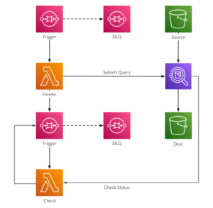
One solution is to add another SQS queue, on which you write the query’s execution ID. That queue then triggers another Lambda to check on the query execution. If it hasn’t finished yet, you can abort the Lambda, which will requeue the message, and eventually send it to a dead-letter queue. On failure, the Lambda can write a message to SNS, will then broadcast the problem to whoever is responsible.
The problem with this architecture is that it doesn’t scale: if you have one long-running query then it’s fine. If you have two or three then maybe it’s OK to duplicate the entire stack using CloudFormation or your IaC tool of choice. But at some point you’ll be overwhelmed with duplicated components, and start thinking of ways that you can refactor. Eventually, you’ll end up writing your own orchestration framework.
Rather than do this, use an existing orchestration framework such as Airflow, especially if it’s already part of your toolbox. Airflow has operators and sensors for working with AWS, and I’ve used them in an example DAG that performs the steps listed above. But Airflow isn’t the only orchestration framework available, and the code to execute a query and wait for it to complete isn’t complex; you could use the framework just to execute a fully self-contained task.
Conclusion
I like SQL. There are some tasks that it’s not very good at, but it’s great for data transformations. The very nature of a SQL query seems more understandable than transforms performed in code. Although I have seen some horrendous SQL queries, I’ve seen far more unintentionally obfuscated code (I’m sure it was crystal clear to the person who wrote it, when they wrote it).
Athena also offers improved performance versus other transformations methods. The CTAS query for a single month of aggregated CloudTrail data took around 7 seconds, versus 40+ seconds for the fully-programmatic Lambda in my previous post. More dramatic, Athena was able to aggregate and transform a month’s worth of raw CloudTrail data, 147,000 files, in under a minute. The combined stage-1 and stage-2 aggregations would take nearly two hours if executed sequentially.
The reason that Athena is so fast is that it brings a lot of readers to the table. While any individual reader may be limited in how many files it can process per second, a hundred readers running in parallel completely changes the outcome. Athena doesn’t report how many workers it uses for any given query, but clearly it’s a lot (my best guess, for my queries, is 50).
If you’d like to experiment more, I’ve added a “stage-3” to the CloudTrail aggregation example.