
I first experienced unbalanced data in a data warehouse thirty years ago. I was working for a mutual fund company, and something like a quarter of our customers had one well-known fund in their portfolio. Our data warehouse was a 64-processor machine, and most queries would take seconds or minutes to run. Except for some queries that involved this particular fund; those would take hours if we let them run.
A couple of years ago, I saw a similar problem with a dataset on Redshift. And while not as dramatic as the thirty year old example, it still increased query runtime. Not just for that query, but for everything else that ran on the machine. This post looks at that issue, its underlying causes, ways to diagnose similar problems, and how to work around the issue.
Decision Support versus Online Transaction Processing
Most relational (and NoSQL) databases are optimized for online transaction processing (OLTP), in which the application changes only a few rows at a time. For example, when a bank customer moves money between their accounts, the banking core application will add rows to a transaction table and probably update rows in an account summary table. That customer might then look at their per-account transaction history, which shows a dozen or so transactions since their last statement.
Even though thousands of customers might be doing the same thing every day, collectively they only “touch” a small percentage of the rows in the database. Moreover, such queries typically retrieve all columns from the tables they access: customers want to see the payee or check number, along with date and amount.
Decision support queries, by comparison, typically look at large chunks of the data, but only limited columns. For example, a compliance official might want a list of all customers with multiple $10,000 transactions in the past month. Or a marketing analyst might want to see the number of customers who either make > 10,000 transactions or have an aggregate transaction amount > $1,000,000 in a year. The latter query might look like this:
select  count(distinct c.id)
from    customers c
join    transactions t on t.customer_id = c.id
where   t.transaction_date between '2022-01-01' and '2022-12-31'
group   by c.id
having  count(*) > 10000
or      sum (t.amount) > 1000000;
Queries like this can be performed by any database engine, decision support or OLTP. But …
An OLTP transactions table almost certainly doesn’t have an index that directly supports the transaction_date predicate, so the query engine will read every row from the table to find those that match. And since OLTP databases typically store all of the fields of a row together, that means reading every block in the (presumable large) transactions table. Furthermore, the query engine will need to traverse an index on the customers table for each row selected from transactions, to satisfy the join (and we hope that it’s smart enough that it won’t actual read the customers table!).
A decision support database, by comparison, typically uses columnar storage: all of the values for a single column are stored together, so the engine only reads the data for columns directly referenced by the query. And it’s likely to be physically ordered by transaction date, so the optimizer can ignore large chunks of the table. Finally the join between customers and transactions will be performed with an efficient hash-based or sort-merge join, again involving just the join columns, and without involving any indexes.
But the most important optimization that a decision support database makes is to store the data on multiple nodes, and parallelize the query. Each “worker” node looks only at the data it holds; the results from those workers are sent to a “leader” node for aggregation. This is far more efficient than the single-node OLTP database; adding nodes scales query performance almost linearly.
However, this means that you must think about how to distribute data between worker nodes.
The Problem
If you have one large fact table, and your queries are just slices of that table, then there’s no need to specify a distribution key; let the engine distribute the rows randomly. And in this scenario you will never see an unbalanced query.
But if you are trying to maintain a relational structure, with joins between tables, then picking the right distribution key becomes critical. Decision support databases like Redshift can only join rows that are on the same node. If you join on a column that’s not the distribution key, then the engine must redistribute the rows from one (or both!) of the tables so that it can perform the join.
People who are new to decision support databases often distribute their tables using the primary key of the source data. However, that’s rarely the right approach. In the case of the transactions table, each row probably has unique ID as its primary key. If you distribute based on that ID, then the table (or the subset of selected rows) must be redistributed for every query that joins to another table. Instead, if most of your queries join transactions to customers, you should use customer_id as the distribution key for both tables (and, if transactions doesn’t have a customer_id column, you might have to add one during ETL … but that’s a topic for another post).
Even if you pick a key that suits your joins, you can still get poorly performing queries. If one customer, for example, had significantly more transactions than the others, then the worker holding that customer’s data would have to process more data than the other workers — it becomes a “hot” node.
A Case Study
While this situation is unlikely to ever happen with bank account transaction data, it can easily happen with the “clickstream” data that shows a user’s actions on a website, and this was the case with a project that I worked on a couple of years ago.
The team used Segment “Track” events to record user actions, and distributed that data on the user_id field. However, the data included actions by “anonymous” users in addition to logged-in users. And for those users, the user_id field contained null; the anonymous_id field held the actual identifier, a UUID.
When the app launched, this wasn’t a problem. After a year, and several hundred million Track events, user-based queries started to show distinct performance problems.
Diagnosing Hot Nodes
The easiest way to diagnose unbalanced data is with CloudWatch:
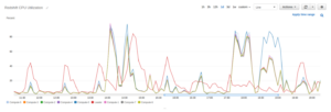
This graph is the CPU utilization by node, for an eight-node cluster. On the right side, starting at the 18:30 timestamp, you can see that the blue line representing node 0 is significantly higher than the lines representing the other worker nodes. This is the smoking gun for an unbalanced query: one node doing more work than the others. And it’s node 0, which is where rows with null distribution keys end up.
However, unless you habitually watch CloudFormation dashboards, you’re not likely to see this smoking gun (at the time, I was working backward from long-running queries).
What you can see at any time is the distribution of data in your tables, available from the STV_BLOCKLIST system table. This query shows your top 20 tables based on the difference of node 0 to other nodes:
with space_used (schemaname, tablename, mbytes, avg_node_mbytes, node0_mbytes) as
        (
        select  trim(pgn.nspname),
                trim(tbl.name),
                sum(bl.mbytes),
                sum(bl.mbytes) / (select count(distinct node) from stv_slices),
                sum(case when bl.node = 0 then bl.mbytes else 0 end)
        from    (
                select  id, name, sum(rows) as rows
                from    STV_TBL_PERM
                group by db_id, id, name
                ) as tbl
        join    PG_CLASS as pgc on pgc.oid = tbl.id
        join    PG_NAMESPACE as pgn on pgn.oid = pgc.relnamespace
        join    (
                select  bl.tbl, s.node, count(*) as mbytes
                from    stv_blocklist bl
                join    stv_slices s on s.slice = bl.slice
                group by bl.tbl, s.node
                ) bl on bl.tbl = tbl.id
        group by 1, 2
        )
select  *
from    space_used
order   by (node0_mbytes - avg_node_mbytes) desc
limit   20;
Here’s an example of running that query. The “balanced” table is distributed on a column containing a UUID (so it should be evenly divided between nodes). The “unbalanced” table contains the same data, but 25% of the rows have a null in the distribution field.
 schemaname  |      tablename      | mbytes | avg_node_mbytes | node0_mbytes
-------------+---------------------+--------+-----------------+--------------
 public      | unbalanced          |   3904 |             976 |         1336
 public      | balanced            |   4687 |            1171 |         1132
Dealing With Unbalanced Data
As a first step, if you know that you have data with nulls in its distribution key, write queries that explicitly exclude those values. Yes, I can hear all of the data scientists gasping in horror. But the truth is, in many if not most cases you don’t need to mix known and unknown users in the same query – and when you do, a UNION ALL can recombine separate queries in a performant way. You can also use NVL to combine the user_id and anonymous_id columns before joining (assuming their values don’t overlap).
You can also write your queries to minimize the number of rows subject to imbalance. Going back thirty years, many of the problem queries involving “that fund” joined to a (relatively large) table of attributes, which would then be used as grouping columns for the output. Breaking the query in two solved that problem: the first query would aggregate by fund (which could be performed in parallel and resulted in a very small number of rows), and the second joined to the attributes table to produce final output.
While these solutions can improve your query performance, they don’t impact unbalanced disk storage, which can become a hard limit on your data warehouse. Most Redshift node types have a fixed disk allocation; as your unbalanced data grows, you’ll be forced to change to a node type with more storage capacity, even if it’s not optimal for your workload.
In the “anonymous user” scenario, I believe that the best solution is is to combine these identifiers into a single column, with a flag to indicate which type of ID you’re working with. Queries that just care about authorized users can include a WHERE condition on that flag field, while queries over the whole dataset can run as-is. The one caveat is that you must ensure that the two IDs have non-overlapping values.
And lastly, you might need to separate your data into multiple tables, distributed on different columns. Again, in the rare cases when you need to combine them, UNION ALL is your friend.
Conclusion
Decision support databases have a number of quirks that are not obvious to the casual user, particularly someone coming from an OLTP background. It’s critical to understand how your data is stored, and how it’s used in a query. It may make the difference between writing a query that takes seconds to run, and one that takes hours.
Can we help you?
Ready to transform your business with customized data engineering solutions? Chariot Solutions is your trusted partner. Our consultants specialize in managing software and data complexities, tailoring solutions to your unique needs. Explore our data engineering offerings or reach out today to discuss your project.