Food for thought
Very simply put, the idea behind backpressure is the ability to say "hey slow down!". Let's start with an example that has nothing to do with software:
Imagine you own a factory that produces doughnuts (lucky you!) and just signed a contract with the largest grocery chain in the Northeast US. To increase output, you decided to overhaul your existing factory and open a new one. Late Monday evening you get a text "Emergency! Get to the factory now!". It turns out doughnuts were being produced 5% faster than they could be glazed and packaged. Needless to say, there was a big, tasty mess to clean up, one of the factories had to be temporarily shut down, and you couldn't fulfill your contract.
Misconfiguration can literally wreak havoc. To make matters worse, the glazer couldn't react by signalling "hey you, slow down!". Even if it could, it didn't have a way to hold on to some extra doughnuts or throw them into a plain donut bin while things slowed down. Being able to signal backpressure and handle temporary bursts is critical in building resilient systems.
Today we'll demonstrate backpressure in Akka Streams (note this is not an intro to Akka Streams itself).
Basic Layout
Our examples will follow the structure shown below:
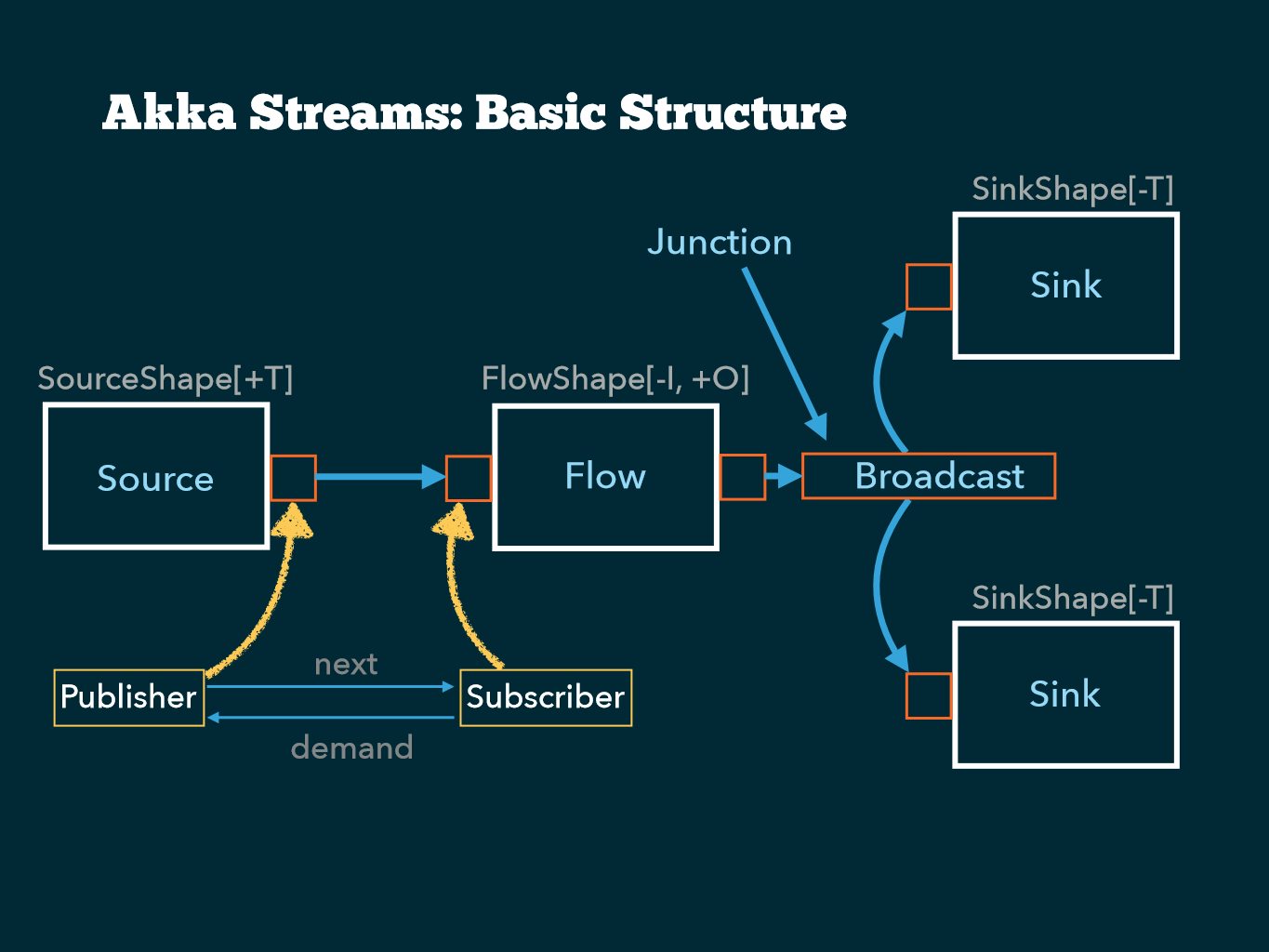
We'll produce a single sequence of integers (source), transform it by computing the factorial of each integer, print them to standard output (flow), and also write out the sequence to two files (broadcast to sinks). The following code does exactly that (please check out this Github repo and use sbt run or fire up your favorite IDE):
object StreamApp  {
  def lineSink(filename: String): Sink[String, Future[IOResult]] = {
    Flow[String]
      .alsoTo(Sink.foreach(s => println(s"$filename: $s")))
      .map(s => ByteString(s + "\n"))
      .toMat(FileIO.toFile(new File(filename)))(Keep.right)
  }
  def main(args: Array[String]): Unit = {
    implicit val system = ActorSystem("streamapp")
    implicit val materializer = ActorMaterializer()
    val source: Source[Int, NotUsed] = Source(1 to 100)
    val factorials: Source[BigInt, NotUsed] =
      source.scan(BigInt(1))((acc, next) => acc * next)
    val sink1 = lineSink("factorial1.txt")
    val sink2 = lineSink("factorial2.txt")
    val slowSink2 = Flow[String].via(Flow[String]
      .throttle(1, 1.second, 1, ThrottleMode.shaping))
      .toMat(sink2)(Keep.right)
    val bufferedSink2 = Flow[String].buffer(50, OverflowStrategy.dropNew)
      .via(Flow[String]
      .throttle(1, 1.second, 1, ThrottleMode.shaping))
      .toMat(sink2)(Keep.right)
    val g = RunnableGraph.fromGraph(GraphDSL.create() { implicit b =>
      import GraphDSL.Implicits._
      val bcast = b.add(Broadcast[String](2))
      factorials.map(_.toString) ~> bcast.in
      bcast.out(0) ~> sink1
      bcast.out(1) ~> sink2
      ClosedShape
    })
    g.run()
  }
}
- A range of Ints from 1 to 100 is turned into a
Source[Int, NotUsed]. A source produces values of a specified type. Source[Int, NotUsed]is transformed into a stream of factorials (Source[BigInt, NotUsed]) via thescanmethod- A standalone flow of Strings (not connected to a source and a sink) is defined in the
lineSinkmethod: themapmethod adds a newline and converts the String to a ByteString - This
Flow[String]is then attached to an asynchronous File based Sink via thetoMatmethod. Note the final return typeSink[String, ...] - Two sinks are created by calling
lineSink
These are then assembled into the topology shown above:
RunnableGraph.fromGraphtakes a graph (aka topology). AClosedShapesimply means all inputs and outputs are connected (to sources, sinks, or other flows). Once closed, it is said to be runnable.- The
factorialssource is converted to Strings and then piped to the input of aBroadcast(junction) with 2 branches. - Each branch of the broadcast, identified by a zero-based index, is piped to a different sink.
- Finally, the resulting
RunnableGraphis run. Until the graph is actually run, it is just a blueprint (i.e. no operations have executed).
When we run the program, this is the first eight lines of output:
factorial1.txt: 1
factorial2.txt: 1
factorial1.txt: 1
factorial2.txt: 1
factorial1.txt: 2
factorial2.txt: 2
factorial1.txt: 6
factorial2.txt: 6
This is the magic behind the alsoTo method on Flow. It tells the Flow to also send the elements being produced at that point to another Sink, without changing the flow (i.e. the alsoTo method returns back the Flow). We're cleverly using alsoTo and println to peek into the stream.
So when does backpressure come into play? How is it signaled? What are some ways of handling it? Let's answer these questions via simple examples.
Fast Producer, Fast Consumers
When we run the code as is, we see the output rapidly alternate between factorial1.txt and factorial2.txt, seemingly at the same rate. In this case, both consumers are able to process the data at the rate the source produces it (assuming no major disk I/O contention or problems). Everyone is happy and no doughnut mess.
Fast Producer, Fast and Slow Consumers
Let's make one of the consumers slow. We can do this by forcing one of the sinks to only process one element per second. This is called throttling. Below is the line that creates such a sink:
val slowSink2 = Flow[String]
  .via(Flow[String]
  .throttle(1, 1.second, 1, ThrottleMode.shaping))
  .toMat(sink2)(Keep.right)
When we run this example, the behavior of the output is not what you probably expect. Writes to both factorial1.txt and factorial2.txt are slowed down by the same amount.
factorial1.txt: 1
factorial2.txt: 1
**one second delay**
factorial1.txt: 1
factorial2.txt: 1
**one second delay**
factorial1.txt: 2
factorial2.txt: 2
**one second delay**
factorial1.txt: 6
factorial2.txt: 6
Why do both consumers get slowed down? In fact, what's happening is the source itself is being slowed down. The slow sink is (asynchronously) telling the source how much it can process — demand — one element in this case. It updates this demand when its ready to process again — after one second (in real systems, a producer may not halt but be able to buffer up to a certain point before sending – think of TCP sockets). Put succinctly, the slow sink is signaling backpressure up to the source. The glazer is able to react and slow down the production line.
Fast Producer, Fast and Slow Consumers with buffering: OverflowStrategy.dropNew
What happens if our slow sink can buffer a preconfigured number of elements (for example because it knows it may be slower)?
val bufferedSink2 = Flow[String]
   .buffer(50, OverflowStrategy.dropNew)
   .via(Flow[String]
   .throttle(1, 1.second, 1, ThrottleMode.shaping))
   .toMat(sink2)(Keep.right)
factorial1.txt: 1
factorial2.txt: 1
factorial1.txt: 1
factorial1.txt: 2
factorial1.txt: 6
...
factorial1.txt: 93326215443944152681699238856266700490715968264381621468592963895217599993229915608941463976156518286253697920827223758251185210916864000000000000000000000000
factorial2.txt: 1
**one second delay**
factorial2.txt: 2
**one second delay**
factorial2.txt: 6
**one second delay**
factorial2.txt: 24
**one second delay**
...
factorial2.txt: 1551118753287382280224243016469303211063259720016986112000000000000
The writes to factorial1.txt are not slowed down at all. That can only mean the source continues producing as fast as it can — backpressure has not been signaled. That's because the slow consumer immediately buffers ("absorbs") up to 50 elements, giving a chance for the source to continue chugging along. However, factorial2.txt ends up stopping at the factorial of 51, with a second delay between each element. With OverflowStrategy.dropNew, new elements are dropped while a buffer is full. In this example, since the producer is so much faster than the throttled consumer, it produces all the remaining elements while the buffer is still full — they get dropped. This amounts to throwing away the rest of the doughnuts (or putting them into an unglazed doughnut bin).
Fast Producer, Fast and Slow Consumers with buffering: OverflowStrategy.backpressure
I'm really not happy with the prospect of losing doughnuts, even if it means we have to slow everyone else down! If we change our buffering strategy to Overflow.backpressure, what do you think will happen? Let's find out.
val bufferedSink2 = Flow[String]
   .buffer(50, OverflowStrategy.backpressure)
   .via(Flow[String]
   .throttle(1, 1.second, 1, ThrottleMode.shaping))
   .toMat(sink2)(Keep.right)
factorial1.txt: 1
factorial1.txt: 1
factorial1.txt: 2
factorial1.txt: 6
factorial1.txt: 24
...
factorial1.txt: 1551118753287382280224243016469303211063259720016986112000000000000
factorial2.txt: 1
factorial1.txt: 80658175170943878571660636856403766975289505440883277824000000000000
**one second delay**
factorial2.txt: 2
factorial1.txt: 4274883284060025564298013753389399649690343788366813724672000000000000
**one second delay**
factorial2.txt: 6
factorial1.txt: 230843697339241380472092742683027581083278564571807941132288000000000000
**one second delay**
factorial2.txt: 24
factorial1.txt: 12696403353658275925965100847566516959580321051449436762275840000000000000
**one second delay**
...
factorial2.txt: 93326215443944152681699238856266700490715968264381621468592963895217599993229915608941463976156518286253697920827223758251185210916864000000000000000000000000
Initially the writes to factorial1.txt are not slowed down (like the first example). However, after the buffer fills up, we see the same behavior we saw with a slow consumer and no buffering. With OverflowStrategy.backpressure, backpressure is signaled up to the source when the buffer becomes full. No data is dropped, but the overall throughput is reduced.
Conclusion
I hope these trivial examples help to illustrate what backpressure is. It allows components in your system to react resiliently (e.g. not consuming an unbounded amount of memory) and predictably, all in a non-blocking manner. Starting with tiny experiments can be a great way to explore a new concept. Okay, time to make the donuts!